The Impact of Financial Statement Integration in Machine Learning for Stock Price Prediction

Author: Febrian Wahyu Christanto, Victor Gayuh Utomo, Rastri Prathivi, Christine Dewi
Journal: International Journal of Information Technology and Computer Science @ijitcs
Article in issue: 1 Vol. 16, 2024.
Free access
In the capital market, there are two methods used by investors to make stock price predictions, namely fundamental analysis, and technical analysis. In computer science, it is possible to make prediction, including stock price prediction, use Machine Learning (ML). While there is research result that said both fundamental and technical parameter should give an optimum prediction there is lack of confirmation in Machine Learning to this result. This research conducts experi-ment using Support Vector Regression (SVR) and Support Vector Machine (SVM) as ML method to predict stock price. Further, the result is compared between 3 groups of parameters, technical only (TEC), financial statement only (FIN) and combination of both (COM). Our experimental results show that integrating financial statements has a neutral impact on SVR predictions but a positive impact on SVM predictions and the accuracy value of the model in this research reached 83%.
Stock Prediction, Technical Analysis, Financial Statement, Support Vector Regression
Short address: https://sciup.org/15018963
IDR: 15018963 | DOI: 10.5815/ijitcs.2024.01.04
Text of the scientific article The Impact of Financial Statement Integration in Machine Learning for Stock Price Prediction
In the capital market, there are two methods used by investors to make stock price predictions, namely fundamental analysis, and technical analysis. The fundamental analysis makes stock price predictions based on an analysis of the company's intrinsic fair value compared to the actual stock price [1]. Fundamental analysis performs quantitative analysis of financial reports. Analysis usually includes things such as income, expenses, assets, and liabilities [2]. On the other hand, technical analysis is based on historical stock prices and movements in the previous period to make predictions of stock prices in the future [3]. Technical analysis uses tools such as stochastic, relative strength index or moving average [4].
In computer science, there is a method to make prediction named machine learning (ML). ML learn from training data to create a model. Based on the model, ML able to pro-duce result when new data supplied [5]. Due its characteristic, ML mostly used in prediction [6] or recognition [7]. Naturally, there are plenty researches in stock price prediction using ML. Another researches use neural network, a method in ML, with technical parameter to predict stock price [8-10]. Another ML methods used in predicting stock price are Support Vector Machine (SVM) [11] and Support Vector
Regression (SVR) [4]. The actual parameters in the research are stock technical indicators, such as Simple Moving Average (SMA) and Relative Strength Index (RSI). Those indicators are formulated from historical stock prices. Some research even make prediction by integrating news sentiment [12] or search trend [13] to the technical parameter.
In predicting stock price, ML can also combine with fundamental parameters. However, SVM [14] and neural network [15] are chosen as the method. The actual parameters in the research are Price to Earning, Book Value to Share and liabilities which are taken from company financial statement. While there is research of that use ML with technical parameter or fundamental parameter, the most used parameter with ML is technical parameter. Fundamental parameter is less preferred in ML. Moreover, combining both technical and fundamental parameter in ML is the least preferred. This is interesting since actually both technical and fundamental parameter should make an optimum prediction [16-18].
From the background above, our major contribution in this research as follows: (1). Our works wants to understand the impact of integrating financial statements to technical parameters in predicting stock price using ML. The method of ML used is SVM and SVR. SVM method used to predict price signal (up or down) while SVR method use to predict the price itself. (2). While the experiment may seem like feature selection method, it actually tries to give a proper confirmation of discussion about technical and fundamental parameter in stock prediction with ML. The rest of this paper contains the materials and methods are explained in section 2. In section 3 describes the result and discussion and section 4 outlines the conclusion and possible future work research.
2. Background 2.1. Support Vector Regression (SVR)
The SVR is a development of the Support Vector Machine (SVM). SVR offers the best balance between empirical noise and model complexity. This is achieved by limiting the SVR regression function to the hyperplane class function and providing a boundary, known as the insensitive tube, around the hyperplane. Moreover, the regression function only relies on a limited set of training data, called the support vector. This support-vector is associated with limiting the optimization problem. Given the form dataset (xi, yi) є RN x R, dual SVR optimization problem can be written in the following formula as.
maximize W ( a , a* ) = -^^( a / - a * ) ( a , - a -WCx), ф(xj)') - e£ -^( a * - a^ + Z™1( a - - a )y < (1)
Subject to
S£ i ( a - a * ) = 0 (2)
Moreover, SVR is capable of performing non-linear regression with kernel tricks. It is done by giving the SVR a special kernel function that maps data from the input field to the high-dimensional feature plane, where linear regression is performed. The kernel functions used usually consist of Linear, Polynomial, and Gaussian [19].
-
2.2. Support Vector Machine (SVM)
The problem of separating the set of training vectors which has 2 separate classes, which can be stated in Formula (3).
(xi,yi),x/ eR",yz e {+1.-1},i = 1,...,n
Where xi is an input vector of n dimension with a real number value and yi is the label that defines the class of xi. A separating hyperplane defined by an orthogonal vector w and a bias b specifying the point satisfies describes in Formula (4).
w. x + b = 0
With parameters w and b limited by Formula mint|w.xt + b| > 1
Then the separator hyperplane must meet the following constraints and show in this Formula.
mint|w.xt + b| > 1
The hyperplane that optimally separates the data is the one that minimizes the value.
ф(w)=-(w.w)
The limitation in Formula (7) can be relaxed by adding variables ζi >= 0, i = 1, 2, … , n. So that Formula (7) becomes Formula (8).
yt(w.xt + b) > 1 - <^t,i = 1,2, ^,п(8)
In this way, the optimization problem becomes Formula (9).
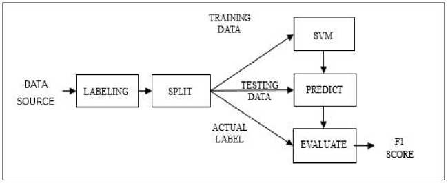
»(w,<) = -(w.w) + CX?=1 In addition, constant C is a positive constant value. The solution of the optimization problem in Formula (10) with the limitations in Formula (9) can be solved using the Lagrange function. L(w, b, a, <, y) = 1 (w. w) + C T=i <, - C Т=М |yt(w. x, + b)-1) + «, | - T=i Yt In Formula (11) the variable αi >= 0, ζi >= 0, i = 1, 2, …, n is the Lagrange factor. Lagrange functions should be minimized against w, b, dan ζi. The classic Lagrange duality allows the main problem in formula (11) to be in the following form which is easier to solve as follows. max [17=1 a, - 1Tw=i а<“уУ<У<(^<. xy)] Which has the following limitations show in Formula (12). £”=1 atyt = 0,0 < at < C, i = 1,2, .„ п It is a classic quadratic optimization problem that allows for unique solutions. The optimal solution will qualify and explain in Formula (13). at[yt(w.xt + b) - 1] = 0, i = 1,2, ^п Formula (14) has a non-zero Lagrange factor if and only if point xi satisfies. yt(w.Xt + b) = 1 This point is called SV. The hyperplane is defined by SV, which is a small subset of the training vector. So that if α_i^* is a non-zero optimal solution, the classification function can be expressed as in Formula (15). /(x) = syn[TP=ia-yt(Xt.x) + b*} The solution to the problem in Formula (15) is b* for each non-zero αi* [20]. 2.3. Root Mean Squared Error (RMSE) and Mean Average Percentage Error (MAPE) 2.4. Research Methods The stock price prediction in this research will be measured using the Root Mean Squared Error (RMSE) and show in Formula (16). RMSE = JlET=i(dt-dt)2 (16) Where T is the amount of data d is the value of factual data and d ^ is the value of predictive data. Another measurement in the research for the stock price prediction is Mean Average Percentage Error (MAPE) and describe in Formula (17). M=7T?.1^| (17) Where n is the amount of data At is the value of factual data and Ft is the value of predictive data [4]. This research uses daily stock price and quarter financial report from companies that listed in LQ45 of Indonesia Stock Exchange (IDX). LQ45 is a compiled list of 45 most liquid companies in IDX. The list is published in IDX official website. Fig.1. SVR diagram The machine learning’s method used are SVR and SVM. The SVR method is shown in Figure 1. In SVR no pre-processing is required to create label since the closing price is the label. Data source is split directly into training data and testing data. SVR creates model based on the training data and uses the model to predict testing data. The prediction is evaluated with the actual label with RMSE [19] / MAPE [21] as the outcome. Fig.2. SVM diagram Moreover, the SVM method is shown in Figure 2. In SVM pre-processing is required to create label. since the closing price is the label. The label is signal up or down. If current’s closing price higher than previous’ closing price, then the signal is up. While if current’s closing price lower than previous’ closing price then the signal is down. Labelled is split into training data and testing data. Further, SVM creates model based on the training data and uses the model to predict testing data. The prediction is validated with the actual la-bel with F1 score as the outcome. Since the data has multiple label, the result from SVR method is evaluated with F1 Score [22]. In this research, there are three groups of features. The first group consists of opening price, highest price, lowest price and closing price of daily stock trading. The first group represents the technical feature. The second group consists of price to earnings ratio (P/E), price to sales ratio (P/S) and price to book ratio (P/B). The second group represents financial statement feature. The third group combines feature from the first group with the second group to represent combination feature. For further reference in the paper, group 1 is labelled TEC, group 2 is labelled FIN and group 3 is labelled COM. All the prediction processes are done five times. However, since the data is originally time-series, the more common random or K-Fold method to create training and testing data considered inappropriate. This research use OSS, which more appropriate to time-series data, with 5 times iteration [23].
3. Results and Discussion Our research work applies LQ45 stock as dataset. However, not all the company has the required financial report. Some of the companies did not publish the financial report in certain period. Some other companies publish incomplete financial report. Due to those reasons, the research use data taken from only 35 companies. Daily stock price ranges from April 2022 to mid-June 2023. Financial report used in this research composed from five quarterly financial reports from Q1 2022 until Q1 2023. Hence, prediction results for each group with SVR method are evaluated. RMSE and MAPE value from all groups are compared. The group with the best prediction is the one with the lowest RMSE or MAPE value. Simple statistic on the frequency of each groups makes the best prediction is created and can be seen on Table 1. Table 1. Best prediction frequency between groups using SVR method Group Frequency (RMSE) Frequency (MAPE) TEC 24 (69%) 23 (66%) FIN 1 (3%) 0 (0%) COM 10 (28%) 12 (34%) Higher value of frequency in Table 1 means better value. Table 1 shows that the order of prediction from the best to the worst is TEC, COM and FIN. The result is consistent in both RMSE and MAPE value. Next examination is calculating the difference between each group. Since from Table 1 it is clear that FIN unable to create competitive prediction and FIN is omitted from the comparison. The difference RMSE and MAPE from each stock prediction in TEC and COM is calculated. The average value from the formula is shown in Table 2. Table 2. Average difference between technical and combination Comparable All Positive Negative RMSE -0.3% 13.5% -5.9% MAPE 1.8% 11.1% -3.1% Furthermore, Negative value in Table 2 means that TEC is better than COM while positive value means that COM is better than TEC. Column 2 shows average from all result. The number in column 1 shows that TEC is better than COM by 0.3% under RMSE evaluation while COM is better than TEC by 1.8% under MAPE evaluation. Besides, it shows that COM and TEC have very small difference and hardly distinguishable. Also, Table 1 shows result that gives TEC as a better group of features compared to COM while the current comparison eliminates the advantage. Further examination held with only averaging positive value and negative value which is shown in column 3 and 4. Both in RMSE and MAPE value, the absolute value of positive average is much higher than the absolute value of negative average. Nevertheless, it means that COM is much better than TEC. By Table 2 only, it may seem the result from column 3 and 4 contradicts with the result from column 2. To explain the finding, Table 1 is brought to analysis. Combining frequency with average difference value, it is clear that TEC is better in higher frequency with small value while COM is better in lower frequency with big value. It is reasonable to conclude that TEC and COM make equal prediction using SVR. Next evaluation is prediction results for each group with SVM method. As the SVR method, F1 value from all groups are compared. The group with the best prediction is the one with the higher F1 value. Simple statistic on the frequency of each groups makes the best prediction is created and can be seen on Table 3. Table 3. Best prediction frequency between groups using SVM method Group Frequency 1 (Technical) 4 (11%) 2 (Financial Statement) 10 (28%) 3 (Combination) 21 (60%) Table 3 shows that prediction with SVM method using combination features is the best while using technical parameters only as features is the worst. Meanwhile, using financial statement only as features comes at second place. Comparing the result from Table 1 and Table 3 is, again, interesting. Since Table 1 gives advantage to group 1 and Table 3 gives advantage to group 3, group 1 and group 3 is compared further. At this point no further comparison can be made since SVR and SVM give incomparable result other than frequency. This research draws same conclusion with previous research [16, 17] that integrating financial statement for stock price prediction has benefit at least in predicting price signal. It also complements [14] which lacks of comparison between the impact of financial statement with the other parameter in stock price prediction. From the prediction that increases with the addition of fundamental parameters, the average error value decreases. The comparison of the reduction in error can be seen in Table 4. Table 4. Prediction error decreasing comparison improves Method Average RMSE -15.88% MAPE -7.73% Table 4 shows a decrease in prediction error when calculated by the RMSE and MAPE methods. The average is taken only from increasing predictions (decreasing error). The decrease in error, when calculated by RMSE, is greater than if calculated by MAPE. This is interesting, because if you look at Table 1. and Table 2. in fact, there are more pre-dictions with decreasing errors when calculated by the MAPE method than when calcu-lated by the RMSE method. From the overall prediction results, the average error value re-duction is taken. The comparison of the reduction in error can be seen in Table 5. Table 5. Error drop comparison Method Average RMSE -11.24% MAPE -5.43% Table 5 shows a decrease in prediction error when calculated by the RMSE and MAPE methods. The average is taken from the overall prediction (error decreases and er-ror increases). From these results, it is clear that the addition of fundamental parameters to stock predictions will reduce errors. If calculated using the RMSE method the decrease was 11.24%, whereas if calculated using the MAPE method the decrease was 5.43%. In this analysis, it is also suggested that the availability of fundamental data is not as complete as technical data. This study was forced to ignore up to 10 company stocks for reasons of incomplete fundamental data. Even for analyzed company stocks, the actual use of fundamental data is not entirely correct. Prediction of stocks with fundamental analysis usually has a long-term time horizon (more than 5 years). Data in this study were limited to 15 months. This data limitation is felt to contribute to the insignificant reduction in prediction errors. Testing for accuracy is carried out using a confusion matrix with reference to four general conditions used as benchmarks in this test, namely True Positive (TP) is the condition when the system detects a financial statement in prediction method has positive impact, True Negative (TN) is the situation when the system detects the condition of the financial statement in prediction method has neutral impact, False Positive (FP) is the condition when the system does not detect the financial statement in prediction method has positive impact, and False Negative (FN) is the condition when the system does not detect the financial statement in prediction method has neutral impact [23-25]. Carrying out 30 trials, the system predicted that 15 financial statement trials in the prediction method had positive impact and 2 positive impacts were predicted not to be detected. There are 13 experiments when the system does not detect the financial statement in prediction method has positive impact. The model also predicts that there are 3 conditions when the system does not detect the financial statement in prediction method has neutral impact. This statement can be seen in Table 6 below. Table 6. Confusion matrix N = 30 Actual Positive (+) Actual Negative (-) Positive Prediction (+) 15 TP 3 FP Negative Prediction (-) 2 FN 10 TN Based on Table 6, 30 experiments have been carried out, so the actual positive and positive predictions are 15 TP, the actual negative and positive predictions are 3 TP, the actual positive and negative predictions are 2 FN, and the actual negative and negative predictions are 10 TN. Once the amount of correctly predicted and incorrectly predicted data is known, calculations can be carried out to determine the accuracy, precision and recall of all the data. After knowing the amount of data from positive actuals, negative actuals, positive predictions and negative predictions, calculations can be carried out in Table 7 below to determine the accuracy, precision and recall of the financial statement in prediction method has positive impact. Table 7. Confusion matrix calculation results Parameters Actual and Prediction (%) Accuracy 0.8333 Precision 0.8333 Recall 0.8823 Based on experiments from Table 7, the results of the confusion matrix calculation for detecting financial statements in the prediction method obtained an accuracy value of 83.33%, then a precision value of 83.33% was obtained, and a recall value of 88.23% was obtained. Based on the results obtained, it can be concluded that the accuracy, precision and recall values are good, so this model can make predictions well.
4. Conclusions Prediction with SVR method predicts the stock price itself. This research finds that integrating financial statement with technical parameter to SVR prediction has mixed impact. From frequency point of view, the integration failed to improve the prediction. Prediction with technical parameter only gives the best result (69% RMSE and 66% MAPE) compared to combination features (28% RMSE and 34% MAPE) and financial report only (3% RMSE and 0% MAPE). While from RMSE and MAPE differences, the integration gives an indistinguishable result between combination features (better 1,8% MAPE) and technical parameter (better 0.3% RMSE). However, judging the overall result, this research concludes that integration of financial statement in prediction with SVR method has neutral impact. Another prediction with SVM method predicts the price signal (up or down). From the result, combination features make the best prediction at the highest frequency (60%) compared to financial statement (28%) and technical parameter (11%). The result evaluated with F1-Score. The conclusion is integration of financial statement in prediction with SVM method has positive impact and the accuracy value of the model in this research reached 83%. Limited availability of fundamental data limits the prediction process. In our future works, we will conduct research with more complete fundamental data (covering at least 5 years) is expected to provide a more precise picture of predictions using combined technical and fundamental parameters.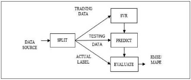
References The Impact of Financial Statement Integration in Machine Learning for Stock Price Prediction
- S. M. Bartram and M. Grinblatt, “Agnostic fundamental analysis works,” J. financ. econ., vol. 128, no. 1, pp. 125–147, Apr. 2018, doi: 10.1016/j.jfineco.2016.11.008.
- S. Muhammad, “The Relationship Between Fundamental Analysis and Stock Returns Based on the Panel Data Analysis; Evidence from Karachi Stock exchange (KSE),” Res. J. Financ. Account. www.iiste.org ISSN, vol. 9, no. 3, pp. 84–96, 2018.
- I. K. Nti, A. F. Adekoya, and B. A. Weyori, A systematic review of fundamental and technical analysis of stock market predictions, vol. 53, no. 4. Springer Netherlands, 2020.
- B. M. Henrique, V. A. Sobreiro, and H. Kimura, “Stock Price Prediction using Support Vector Regression on Daily and up to the Minute Prices,” J. Financ. Data Sci., vol. 4, no. 3, pp. 183–201, 2018, doi: 10.1016/j.jfds.2018.04.003.
- S. Huang, C. A. I. Nianguang, P. Penzuti Pacheco, S. Narandes, Y. Wang, and X. U. Wayne, “Applications of support vector machine (SVM) learning in cancer genomics,” Cancer Genomics and Proteomics, vol. 15, no. 1, pp. 41–51, 2018, doi: 10.21873/cgp.20063.
- L. H. Li, C. Y. Lai, F. H. Kuo, and P. Y. Chai, “Predictive Maintenance of Vertical Lift Storage Motor Based on Machine Learning,” Int. J. Appl. Sci. Eng., vol. 16, no. 2, pp. 109–118, 2019, doi: 10.6703/IJASE.201909_16(2).109.
- Y. C. Tsai and T. N. Chou, “Deep Learning Applications in Pattern Analysis Based on Polar Graph and Contour Mapping,” Int. J. Appl. Sci. Eng., vol. 15, no. 3, pp. 183–198, 2018, doi: 10.6703/IJASE.201812_15(3).183.
- O. B. Sezer, M. Ozbayoglu, and E. Dogdu, “An Artificial Neural Network-based Stock Trading System Using Technical Analysis and Big Data Framework,” Procedia Comput. Sci. 114, no. 2, pp. 1–4, 2017.
- A. Munde, A. Jadhav, H. Kaute, and A. Gosavi, “Automated Stock Trading Using Machine Learning,” SSRN Electron. J., 2021, doi: 10.2139/ssrn.3772584.
- M. Agrawal, A. U. Khan, and P. K. Shukla, “Stock Price Prediction using Technical Indicators : A Predictive Model using Optimal Deep Learning,” Int. J. Recent Technol. Eng., vol. 8, no. 2, pp. 2297–2305, 2019, doi: 10.35940/ijrteB3048.078219.
- E. Ahmadi, M. Jasemi, L. Monplaisir, M. A. Nabavi, A. Mahmoodi, and P. Amini Jam, “New Efficient Hybrid Candlestick Technical Analysis Model for Stock Market Timing on the Basis of the Support Vector Machine and Heuristic Algorithms of Imperialist Competition and Genetic,” Expert Syst. Appl., vol. 94, pp. 21–31, 2018, doi: 10.1016/j.eswa.2017.10.023.
- G. Attanasio, L. Cagliero, P. Garza, and E. Baralis, “Combining News Sentiment and Technical Analysis to Predict Stock Trend Reversal,” IEEE Int. Conf. Data Min. Work. ICDMW, vol. 2019-Novem, no. iii, pp. 514–521, 2019, doi: 10.1109/ICDMW.2019.00079.
- P. F. Pai, L. C. Hong, and K. P. Lin, “Using Internet Search Trends and Historical Trading Data for Predicting Stock Markets by the Least Squares Support Vector Regression Model,” Comput. Intell. Neurosci., vol. 2018, 2018, doi: 10.1155/2018/6305246.
- M. Nabipour, P. Nayyeri, H. Jabani, S. Shahab, and A. Mosavi, “Predicting Stock Market Trends Using Machine Learning and Deep Learning Algorithms Via Continuous and Binary Data; A Comparative Analysis,” IEEE Access, vol. 8, pp. 150199–150212, 2020, doi: 10.1109/ACCESS.2020.3015966.
- Y. Huang, L. F. Capretz, and D. Ho, “Neural Network Models for Stock Selection Based on Fundamental Analysis,” 2019 IEEE Can. Conf. Electr. Comput. Eng. CCECE 2019, no. May, pp. 1–4, 2019, doi: 10.1109/CCECE.2019.8861550.
- B. A. Elbialy, “The Effect of Using Technical and Fundamental Analysis on the Effectiveness of Investment Decisions of Traders on the Egyptian Stock Exchange,” Int. J. Appl. Eng. Res., vol. 14, no. 24, pp. 4492–4501, 2019.
- Q. Hu, S. Qin, and S. Zhang, Comparison of Stock Price Prediction Based on Different Machine Learning Approaches, vol. 3. Atlantis Press International BV, 2023.
- E. Mangortey et al., “Application of machine learning techniques to parameter selection for flight risk identification,” AIAA Scitech 2020 Forum, vol. 1 PartF, no. January, 2020, doi: 10.2514/6.2020-1850.
- H. Muthiah, U. Sa, and A. Efendi, “Support Vector Regression (SVR) Model for Seasonal Time Series Data,” Proc. Second Asia Pacific Int. Conf. Ind. Eng. Oper. Manag., no. September 14-16, 2021, pp. 3191–3200, 2021.
- E. Sariev and G. Germano, “An innovative feature selection method for support vector machines and its test on the estimation of the credit risk of default,” Rev. Financ. Econ., vol. 37, no. 3, pp. 404–427, 2019, doi: 10.1002/rfe.1049.
- E. Fradinata, Z. M. Kesuma, S. Rusdiana, and N. Zaman, “Forecast Analysis of Instant Noodle Demand using Support Vector Regression (SVR),” IOP Conf. Ser. Mater. Sci. Eng., vol. 506, no. 1, 2019, doi: 10.1088/1757-899X/506/1/012021.
- B. Wang, C. Li, V. Pavlu, and J. Aslam, “A Pipeline for Optimizing F1-Measure in Multi-label Text Classification,” Proc. - 17th IEEE Int. Conf. Mach. Learn. Appl. ICMLA 2018, pp. 913–918, 2019, doi: 10.1109/ICMLA.2018.00148.
- C. Bergmeir, R. J. Hyndman, and B. Koo, “A note on the validity of cross-validation for evaluating autoregressive time series prediction,” Comput. Stat. Data Anal., vol. 120, no. April, pp. 70–83, 2018, doi: 10.1016/j.csda.2017.11.003.
- I. Düntsch and G. Gediga, “Confusion Matrices and Rough Set Data Analysis,” J. Phys. Conf. Ser., vol. 1229, no. 1, 2019, doi: 10.1088/1742-6596/1229/1/012055.
- I. Markoulidakis, I. Rallis, I. Georgoulas, G. Kopsiaftis, A. Doulamis, and N. Doulamis, “Multiclass Confusion Matrix Reduction Method and Its Application on Net Promoter Score Classification Problem,” Technologies, vol. 9, no. 4, 2021, doi: 10.3390/technologies9040081.
