The numerical probabilistic approach to the processing and presentation of remote monitoring data

This contributes to the development of new numerical methods and approaches to representation, numerical modeling and data analysis of remote monitoring in terms of different types of uncertainty. The variety of ways of presenting data determines the choice of methods of processing, modeling and analysis. The classical approach to data processing and analysis usually assumes that each value is the only point in n -dimensional space Rⁿ [1]. In addition to such data in many practical problems of storage, processing, analysis, have to deal with “multi-value” data, examples of which include: a list of values, interval date and other types. A more complex type is modal - valued data containing the probability of weight, or any other related matter. A good example of a modal-valued data is a histogram. Such data gets to a data class, called “symbol” data [1]. An important difference between the symbol data is the presence of internal structures. It is does not apply the classical statistical theory and methods of data processing and analysis for symbolic data. Therefore, development of new methods for the analysis of such data and construct mathematical fundamentals are more important. Note that the large amount of information on the one hand, provides a more precise description of the object of research, on the other hand makes the difficulties for the search for solutions to the challenge. One way to solve this problem is to use a variety of data preprocessing procedures. For example, the aggregation method is a method of compressing large data. Procedures for the conversion of input data arrays into arrays of smaller dimension while maintaining useful information are the basis of aggregation. This article discusses the methods of presenting the data as a histogram, polygons, splines, histogram time series. On the basis of data representation methods we are solving the problem of data aggregation. Applying the numerical probabilistic analysis we are studying the existing relationships and trends in the data and are considering the questions of construction histogram regression models. For this purpose, the aggregated data we are presenting in the form of histograms and polygons.

Data representation

We will use a numerical probabilistic analysis for the processing and analysis of remote monitoring data, using such representation as histograms, polygons and splines. Histograms are one of the best known methods for presenting data.

Histograms. The histogram is called a random variable density which is represented piecewise constant function. Histogram P is defined grid { x_t | i = 0 , ..., n }, on each interval [ x - 1 , x i ], i = 1 , ..., n histogram takes constant value of p i . Histograms are widely used for the processing and analysis of remote sensing data. For example, in [2] is considered the problem of the study of natural processes on the basis of space and ground monitoring data. In addition to histograms we discuss the piecewise linear functions (polygons) and splines.

The piecewise linear function (Frequency Polygons). Piecewise linear functions can considered as a tool of approximation of the density function random variable. A piecewise linear function is a function composed of straight-line sections. The frequency polygon (FP) is a continuous density estimator based on the histogram. In one dimension, the frequency polygon is the linear interpolant of the midpoints of an equally spaced histogram.

Spline. A spline is a sufficiently smooth polynomial function that is piecewise-defined, and possesses a high degree of smoothness at the places where the polynomial pieces connect (which are known as knots). We will consider the probability density of the random variables are approximated spline.

Data aggregation

Aggregation can be considered as a data conversion process with a high degree of detail to a more generalized representation, by computing so-called aggregates or values obtained as a result of this conversion to a certain set of facts related to a specific dimension. An example of such procedures is a simple summation, calculation of the average, median, mode and range of maximum or minimum values. Application of aggregation procedures has its own advantages and disadvantages. Detailed data are often very volatile due to the impact of different random factors. It is making difficulties for detecting the general trends and patterns. It is important to bear in mind that the use of such procedures as averaging procedure, the exclusion of extreme values (emission), the smoothing procedure can lead to loss of important and considerable part of the useful information.

There are two typical situations where this happens [3]:

• •    If a variable is measured through time for each individual of a group, and the interest does not lie in the individuals but in the group as a whole. In this case, a time series of the sample mean of the observed variable over time would be a weak representation.

• •    When a variable is observed at a given frequency (say minutes), but has to be analyzed at a lower frequency (say days). In this case, if the variable is just sampled at the lower frequency, or if only the highest and lowest values between consecutive lower-frequency instants are represented (as is done when summarizing the intra-daily behavior of the shares in the stock markets), a lot of information is neglected.

These two situations describe contemporaneous and temporal aggregation, respectively.

Consider the histogram approach to data aggregation. This approach is useful for the following reasons. The histogram can be regarded as a mathematical object that is easy to describe and calculate the mathematical procedures and operations, while maintaining the essence of the frequency distribution of the data.

There is histogram arithmetic [4, 5], which allows you to perform various arithmetic operations on histogram variables, including the operation of calculating the maximum and minimum, raising to a power, the comparison procedure. Currently, histograms are used extensively in various fields. For example, histograms are widely used in databases and in the problems of approximating data, pattern recognition. Histograms are widely used in image processing problems, since the histogram characterizes the statistical distribution the number of pixels in the image depending on their values.

We note an important property of the histogram, which is associated with the aggregation of information. Note that the histogram adequately represents the distribution of random variables. Despite its simplicity, the histogram covers all possible ranges of probability density function estimation. Simple and flexible structure of histograms greatly simplifies their use in numerical calculations and has a clear visual image, which is useful for analytical conclusions.

Consider one example of a histogram approach to aggregate large amounts of data. Assume that the characteristics is monitored some of the observed object. For clarity, let it be temperature. Monitoring is carried out over the area Ω, which is represented as a union of subareas Ω i . It is assumed that the temperature measurement points distributed uniformly in each of the subareas. Temperature as input parameter of standard model is described to average values x i in the subarea Ω i .

Remote sensing allows you to submit N_i temperature values for each subarea Ω _i . Where i is number of subarea, j is number of measurement. Thus, each x i is represented as an average value

• 1    ^{N i}

  X i ^-

  
  

\ ^xij i J-1

It is proposed to reduce the level of uncertainty in the data and instead of the average values of input parameters to use histogram representation for each subarea.

Consider the histogram P x for the value x . Suppose that for the value x is known sample ( x 1 , x 2 , . , ^X N ). Denote by n J the number members x , of the re-sampling ^{( x} 1 , ^x 2 , . ^X N ) got into interval [ z , -_P z , ], then

• p .   n j .

^J N ⁽ z j - z j -1 )

Thus, for each input variable x i may be known, not only the average value x i but also the histogram P i .

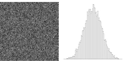
Fig. 1 shows a model example histogram P i by values in a certain area Ω i .

Assume that the area Ω _i is rectangle region. It is composed of 100 × 100 pixels. For each pixel value is put in appropriate value P i,j . For clarity in Fig. 1 values x i,j are shades of gray. Lighter colors correspond to a higher temperature. Thus, the histogram describes the frequency distribution of the temperature into Ω i

Considered approach demonstrates an effective way to aggregate data. So instead of 10⁴ values represented in the subarea Ω i for histogram is used only about 10² values. Moreover, histograms include a lot more information as interval of value change, the mean value, frequency and etc.

The frequency polygon (FP) is a continuous density estimator based on the histogram, with some form of linear interpolation. Transformation histogram in the frequency polygon can be represented graphically Fig. 2. [6].

In one dimension, the frequency polygon is the linear interpolant of the midpoints of an equally spaced histogram.

Theoretical basis of numerical probabilistic analysis

The subject of the NPA is to solve the various problems with data stochastic uncertainties using numerical operations on the probability densities of the random variables and functions with random

a)                                   b)

Fig. 1. a) – subarea Ω i , b) – histogram P i

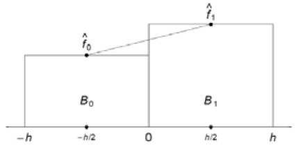
Fig. 2. The frequency polygon in a typical bin, (-h/2; h/2), which is derivedfrom two adjacent histogram bins arguments. To this end, were developed varied tools, including concepts such as arithmetic, histogram, probability, histogram, probabilistic extension, second order histogram, histogram time series.

It is a non-parametric approach can be successfully applied for the probabilistic description of systems as part of an interactive visual simulation, thereby increasing the quality of research systems [4]. In the test cases and some practical problems were proved the advantage of this approach to the Monte Carlo method [5].

Consider the basic theoretical aspects of the NPA. Arithmetic for different data types is one of the important components of numerical probabilistic analysis. NPA-arithmetic reduces the uncertainty level in the data and helps to obtain the additional information on the distribution of random variables. These are operations “+”, “–”, “∙”, “/”, “↑”, “max”, “min”, as well as binary relations “≤”, “≥” and some others. The numerical operations of the histogram arithmetic constitute the major component of NPA.

In [4, 5] developed numerical approaches to the various operations of the histogram variables, including the arithmetic operations, comparison operations, the procedure of calculating the maximum and minimum.

It is noted that the number of arithmetic operations to compute the procedure x * y by the histogram method over the variables x and y is near the order O ( n ²), where n is dimension of the histogram.

A histogram is a piecewise constant function approximates the probability density with an accuracy O (1/ n ). However, even midpoints of histogram are approximated the probability density function with precision O (1/ n 2 ). Consequently, the frequency polygon approximates the function with the accuracy O (1/ n 2 ). Note that the arithmetic complexity does not increase.

Let us consider histogram operations. Let p ( x , y ) be a joint probability density function of two random variables x and y . Let p_z be a histogram approximating the probability density of the operations between two random variables x * y , where * e { +, -,-, /,T }. Then the probability to find the value z within the interval [ z i , z i _{+ 1} ] is determined by the formula [4, 5]

P (zk < z < zk+i) = Jn k p(x,y)dx dy, where Qk = {(x, y) | zk < x * y < zk+1} and the value Pk of the histogram on the interval [zk, zk+1] is defined as

P k = L P ^{( x} ’ у ) ^dx dy ^{/ ( z} k +1 ^{- z} k ) • ^Q k

Then we extend the order relation > e { <,<, >, > } to random variables [7]:

x >  y if and only if x >  y for all x e x , y e y .

If the support of x , y are intersected, then we can talk about the probability of x ^ y

P (x ^ y) = £ p (x, y) dxdy, where Q = {(x, y) | x > y} is the set of points (x, y) e R2 such that x ^ y, p (x, y) is the joint probability density of x, y.

For example, consider the operation max( x , y ). The probability P (max( x , y ) <  z ) is determined by the formula

P ( z ) =[ P ( x , y ) dxdy ,

Q z where Qz = {(x, y) | (x < z) and (y < z)} and the value Pi of the histogram on the interval [zi, zi+1] is defined as

P i = ( P ( z_{i + 1}) - P ( z )) / ( z_{i + 1} - z ) .

Probabilistic extension. One of the most important problems that NPA deals with is to construct probability density functions of random variables. Let us start with the general case where ( x 1 , ..., xn ) is a system of continuous random variables with the joint probability density function p ( x 1 , ._, x n ) and the random variable z is a function f ( x 1 , ..., x n )

z = f ( x i , ..., xn ) .

By probabilistic extension of the function f , we mean the probability density function of the random variable z .

Let us construct the histogram F approximating the probability density function of the variable z. Suppose the histogram F is defined on a grid { z i | i = 0 , ..., n }. The domain is defined as Q i = {( x 1 , ._, x n ) | z i <  f ( x 1 , ..., x n ) <  z i _{+ 1}}. Then the value F i of the histogram on the interval [ z i , z i _{+ 1}] is defined as

By histogram probabilistic extension of the function f , we mean the histogram F constructed according to (1).

Let f ( x 1 ,..., x n ) be a rational function. To construct the histogram F , we replaced the arithmetic operation by the histogram operation, while the variables x 1 , x 2 , …, x n are replaced by the histogram of their possible values. It makes sense to call the resulting histogram of F as natural histogram extension (similar to “natural interval extension”).

Case 1. Let x 1 , ..., x_n be independent random variables. If f ( x 1 , ..., x n ) is a rational expression where each variable x i occurs no more than once, then the natural histogram extension approximates a probabilistic extension.

Case 2. Let the function f ( x 1 ,._, x n ) admit a change of variables, so that f ( z 1 ,._, z k ) is a rational function of the variables z 1 , ._ , z k satisfying the conditions of Case 1. The variable zi is a function of x i , i e Ind i and the Ind i are mutually disjoint. Suppose for each z i it is possible to construct the

– 966 – probabilistic extension. Then the natural extension of f (z1,.„, zk) is approximated by the probabilistic extension of f (x1, ..., xn).

Case 3. We have to find the probabilistic extension for the function f ( x1, x 2 , ..., xn ), but the conditions of Case 2 are not fulfilled. Suppose for definiteness that only x 1 occurs a few times.

If, instead of the random variable x ₁, we substitute a determinate value t , then it is possible to construct the natural probabilistic extension for the function f ( t , x ₂ , ..., xn ).

Suppose that t is discrete random value approximating x ₁ as follows. Let t take the value t_i with probability P i and for each function f ( t i , x ₂ , .„, x n ) it is possible to construct the natural probabilistic extension.

Then the probabilistic extension f of the function f ( x 1 , ..., x n ) can be approximated by the probability density φ as follows [4]

n ф 6)= E p ф i 6 )• i =1

Metrics for the probability density function

Due to the nature of histograms for numerical simulation of histogram regressions will use special approaches to quantify the distances between the probability density function. To this end, consider a few metrics that should be used in the histogram regression models

For this pulpous we consider the metric for the probability density function of the random variables [3]

Let f ( x ) and g ( x ) are two probability density functions. Then distances between f ( x ) and g ( x ) are defined as

P W ( f , g ) = [V ^{- 1}( t ) - G ^{- 1}( t )\dt ,                                                  (2)

P M ( f , g ) = ( J 01 ( F "' ( t ) - G ^{- 1} ( t ))² dt ) 1/ ² ,                                                (3)

respectively, where F ^{- 1} ( t ), G ¹ ( t ) - are the inverse cumulative distribution functions f ( x) and g ( x), respectively.

Let h ( x ) be the histogram. Then distribution functions H corresponding to this histogram can be represented as

H ( x ) = f x h ( ^ ) d ^.

-Ю

Due to the fact that the histogram is the piecewise constant function the calculation of the integral of it is not difficult. As a result, the distribution function is a piecewise linear function. Thus, the metrics (2) or (3) can be interpreted as the area between the distribution functions.

Numerical probabilistic approach to the representation of histogram time series

Histogram time series (HTS) describe the situations where for each time point are known histogram approximation of the probability density function of the studied parameter. It is important to – 967 – note that the forecast on the base of histogram time series presents the approximation of the probability density function of the studied process.

In order to construct the numerical procedures for data aggregation we define the histogram time series as a sequence of probability densities represented in the form of histograms. To construct and study the time histogram series will use tools of numerical probabilistic analysis.

Further based on the NPA and the concept of time histogram series are studied data aggregation tasks and construction the information analytical models.

Decomposition method of histogram time series. Consider the forecasting model construction based on the decomposition method of the histogram time series in the histogram subseries [8].

Denote by h, i = 1,...,Nsome histogram time series. Let for each histogram is defined uniform grid to‘ = {zi, j = 0,..,k}, and values p/, j = 1,..,k. Define by zi,zi,PJi,j = 1,...,k,i = 1,...,N.                                                             (4)

auxiliary histogram time series. Next, consider the approach of building a predictive model based on the decomposition of the time series in the histogram contracts.

To construct the forecast h N _{+ 1} will be used the last d-th values of histogram time series (4).

Thus, using one of the methods for constructing the forecast, we construct values z⁰_{N + 1}, z N _{+ 1}, p N _{+ 1}.

Для гистограммы / J N _{+ 1} определим равномерную сетку to N ^{+ 1} = { z N _{+ 1} , j = 0 ,.., k }

Then, let’s define an uniform grid to N ^{+ 1} = { z^J_{N + 1} , j = 0 ,.., k } for histograms / J N _{+ 1}with values p NN _{+ 1}. The final step in the construction of the forecast will be the normalization of the histogram / J N _{+ 1}

nor 1

hN+1 ’= в hN+1, where zk

в = J ,NX+1(^)d^ .

^zN + 1

k

J 0 N + 1 h N + £) d ^ = 1 .

^zN + 1

Numerical example. Consider the historical data of the maximum temperature in the city of Krasnoyarsk in the last hundred years. Сгруппируем данные по дням и построим соответствующие гистограммы.

To test the decomposition method we take histogram for 21-25 in August. According to the decomposition method we construct twelve auxiliary temporary series. Due to the properties of stationarity to construct forecast for the series z 0 = 6 ° , z ¹⁰ = 35 ° , i = 1,...,5 , is trivial. Using the least squares method to ten subseries p i , j = 1,..., 10 , i = 1,..., 5 , we can build a forecast for August 29th. Fig. 3 is shown the comparison of the true value and the forecast for August 29th. As can be seen from the comparison, the predicted value is well matched with the true value.

Regression Modeling

Regression modeling is research method to identify the existence of the various correlations between input and output data.

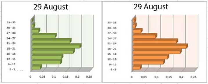
Fig. 3. True and predicted values

Regression analysis includes the following assumptions: the number of observations is sufficient to develop the statistical regularities concerning the factors and their interactions; processed data contains some errors (noise) due to measurement errors, and the influence of random factors; matrix of observations is the only information about the object being studied, the available before the start of the study.

To search for interconnections into remote monitoring data are proposed to use the data aggregation procedure and then to construct the regression model on aggregated data. Regression model to construct on the basis of the histogram data representation we call histogram regression.

Let X = ( x^..., x n )be input data, and Y be output variable. Both, is represented as histogram variables. For X = ( x ₁ ,..., x n ) we now joint probability density function p ( x₁ ,..., x n ).

Similarly classical nonparametric regression can be written for each pair ( X_; , Y i ) by

Y = f (X,, a) + e,, i = 1,..., N,

In the linear case the model can be defined as

n

Y = an + У a x„ + e, i = 1,..., N.

i 0                 j ij i j=1

Thus, for finding the unknown parameters the optimization problem can be represented as

Nn

Ф ( a ) = У p ( Y , a о + У a j X ji ) 2 ^ min, i =1                     j =1

where p be a metric in the space of histograms. Note that due to the nonlinearity of the addition operations under histogram variables to solve the problem (5) can be use the steepest descent method [9]. To calculate the gradient Ф' will use difference derivatives

Ф( a о ,..., a , + h,..., a n ) -Ф( a 1 ,..., a , ,..., a n )

Ф i =                        ,                        ,

h where h be parameter. The initial approximation for the parameters vector can be obtained by solving the regression problem for mathematical expectations (M[Xi], M[Yi]) .

Note that the histogram regression (5) can be regarded as a symbolic regression, since the input and output variables are histogram mathematical objects [1].

Numerical example. Consider the regression model based on the histogram time series aggregation. In this case, we know the measurements of the target variable Y i . Measurements of the input variable will be treated as real.

Consider the temperature data for the last hundred years in the Krasnoyarsk city. For each day from April to October, the data is aggregated in the form of histograms. In this case, the regression model can be represented in the form

Y = Aφ1(t) + Bφ2(t) + Cφ3(t), where A, B, C are the probability density functions, φ1, φ2, φ3 — quadratic functions. Functions A, B, C represented in the form of Hermite cubic splines. Splines are defined by mesh {x1, x2, x3}. Boundary conditions are s(x1) = 0, 5'(x1) = 0, s(x3) = 0, s'(x3) = 0. In addition s'(x2) = 0 and the value of s(x2) chosen from the conditions

J x 3 s ( ^ ) d ^ = 1 .

x ₁

For variable x 1 , x 3 is chosen by regression curves of minimum and maximum temperatures. For x ₂ is chosen by regression curve of average temperatures

In Fig. 4 shows the regression of the probability density functions of the temperature data for the last hundred years in the Krasnoyarsk city, from April to October. Shades of gray define the values of the probability density function. The top and bottom line represents maximum and minimum temperature on each day over the past hundred years respectively. Midline denotes the mean of daily temperature over the last hundred years. Each vertical section is the probability density function of the temperature corresponding to a certain day of the year, according to the observations of the day in the last hundred years. At the first stage, the data presented for each day in a histogram. The regression data are presented in the form of Hermite cubic splines.

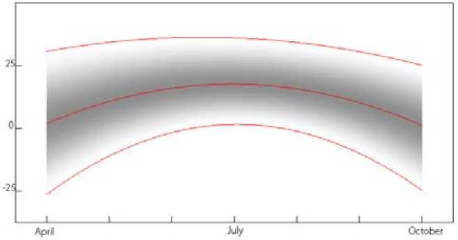
Fig. 4. NPA regression

Conqlusion

Using NPA for preprocessing, processing and modeling of remote monitoring data based on the histogram aggregation contributes to the reliability of the study of natural systems and processes. The spatial and time aggregation procedures helps to reduced the amount of computation in data processing and are an important basis for the extraction of useful knowledge from large volumes of data. Developed on the basis of the NPA submission methods, processing and numerical regression modeling, reduce the level of uncertainty in the information flow, significantly reduce the processing time and the implementation of numerical procedures.

This approach allows the mode of interactive visual modeling to provide the necessary data for operational decision making under remote surveillance techniques and distributed object systems.