The Probabilistic Method for Solving Minimum Vertex Cover Problem Using Systems of Non-linear Equations

Published Online October 2015 in MECS DOI: 10.5815/ijitcs.2015.11.01

One of the main goals of computational complexity theory is to classify computational problems depending on the time and resources required to get their solutions. A computational problem can be viewed as a mathematical object that is described by a collection of questions together with the solutions that satisfy the given properties. The biggest open question of computational theory concerns the relationship between two complexity classes: P and NP [1]. The complexity class P consists of all those problems that can be solved in polynomial time. On the other hand, NP-problems don’t have any efficient polynomial algorithms. Simultaneously, their solutions can still be verified in a reasonable amount of time.

The minimum vertex cover problem (MVCP) for a random graph is called an NP-hard optimization problem

• [2] . An optimization problem is a problem of finding an optimum among all plausible solutions. In the case of MVCP, we are trying to find a vertex cover of smallest possible size. There were many attempts of developing the exact algorithms that allow the problem to be solved in polynomial time. However, both in theory and practice, it is not yet known a method that uses a reasonable amount of time and resources for computing the solution. There are only approximation algorithms that are optimal up to a constant factor [3]. In other words, they yield a vertex cover that has a number of vertices no more than k times bigger in comparison with the minimum cover possible (k is a constant factor of the particular approximation algorithm).

This paper presents the probabilistic method for solving MVCP that has according to the experiment results an improved time complexity and an optimized approximation factor. The first well-known proofs using this method have been presented by Paul Erdős [4]. This method can be described as an efficient technique for proving the existence of mathematical object with certain properties. For this purpose an arbitrary probability space is constructed. Hence, if one chooses a random element form the space, the probability that it will have the desired properties is more than zero.

Over the last few decades this problem has been studied with great attention. It is connected with the fact that MVCP is used in many important and contemporary fields of science and technology. In particular, it is widely used in a telecommunication system monitoring [5] by means of which the areas with slow performance and/or damaged parts of a network can be detected. The minimum vertex cover algorithms, which provide mechanisms and means of detection and analysis of the regions of similarity inside a DNA and relationships between the complete genome sequences [6], play an important role in the biological sequence alignment (protein, DNA, RNA etc.). Such algorithms are also crucial in resolving conflicts of the many problems of computational biology [7].

The importance of this research can be easily seen by examining the coordination of the shared resources in the heterogeneous high performance computing systems, where the choice of the effective and efficient method for solving MVCP plays crucial role in providing stability and obtaining the most cost-efficient level of system performance. It is much easier to expand and manage such systems when dealing with an algorithm that has optimized characteristics taking into account the high intensity task management environment.

• II.    Related Works

In recent years, two main approaches for solving MVCP have been developed: exact evaluation and approximate evaluation. However, it is unlikely that there is an algorithm that solves it exactly in polynomial time unless P = NP. Most of the exact algorithms grow exponentially fast with the problem size for all types of graphs [8]. The distinction between polynomial-time and exponential-time algorithms shows the existence of the two global classes of problems: tractable and intractable.

In practice, the problem that is intractable in infinite input can still be solved by means of some approximation algorithm. The approximation algorithms are often used for solving the optimization problems such as MVCP. One of the most important properties of the approximation algorithm is an approximation factor [9]. An algorithm A is defined to be a p-approximation algorithm for some problem N if on each instance I of this problem it produces a solution s that satisfies the constraints (1).

' fN ( 1 , 5 ) <  p (| I |) ■ OPT ( I ),  if p >  1;

^ fN ( 1 , 5 ) >  p (| I |) ■ OPT ( I ),  if p <  1..

Where OPT (I) is an optimal solution for the problem instance I. It is obvious that the closer p is to 1 the better is the approximation algorithm.

One of the popular 2-approximation algorithms for solving MVCP was discovered by Fanica Gavril and Mihalis Yannakakis [10]. This algorithm considers the maximal matching M of a given graph G and constructs a vertex cover V by selecting all the endpoints of the edges e e G n e e M .

A lot of effort has been put into developing a polynomial time approximation algorithm that is bounded by a constant less than 2. It was even conjectured that no such an algorithm exists [11]. However, improving this 2-approximation algorithm has been finally achieved. One of such recent algorithms has an approximation factor of 2 -©(—) [12]. The semi-definite programming logn relaxation of the vertex covers is used for the reduction of the approximation factor in cases of the weighted and unweighted graphs.

On the other hand, in some cases developing an asymptotically optimal algorithm for solving MVCP has been done taking into account the parameterized complexity [13]. The main idea behind the parameterized complexity is that it is possible to change the structure of the input parameters to get the practical tractability. Hence, on the one hand there is a big set of the input values and on the other hand there is a wide variety of parameters that can affect the overall computational complexity of the algorithm being analyzed. This approach makes it possible to form the more flexible classification of the NP-hard problems in comparison with the classical methodology when complexity is measured in terms of the input size only.

There exist many natural problems that require exponential or worse running time, providing that P ^ NP . However, using a parameterized algorithm allows us to solve such problems efficiently for any input set of values, provided some parameter k is fixed. In other words, if there exists some function f (k) that affects the algorithm complexity and there is a k-parameter that has a relatively small value, there is an algorithm that solves the problems in O(fk) x n^O(1) time, where n is a number of the input values.

Problems that have a fixed k-parameter are called parameterized problems and they belong to the complexity class FPT (fixed-parameter tractable). The vertex cover problem is said to be in this class too. Quite a long time the optimized parameterized algorithms are developed and investigated. At the present time one of the quickest known algorithms solves this problem in O(kn x 1.2738^k) [14], where n is a number of vertices of a random graph and k is the size of the vertex cover.

Among the weakest sides of the approaches to solving MVCP is the lack of attention to the problem of parallelization of operations by means of which the efficiency of execution in a distributed environment could be increased. Many of the known algorithms have too high value of the fixed parameter, which reduces performance of the system.

This article treats and summarizes an approach to solving MVCP for the random graphs that is optimal for using in the distributed environments under high load conditions. The main purpose is to create an algorithm with improved complexity bounds in comparison with the existing methods.

• III.    The Proposed Approach

Let G (V, E) be an arbitrary undirected graph. The term “arbitrary undirected graph” is used here for the sake of the problem formalization. It implies an ordered pair (V, E) where V is a set of vertices and E is a set of edges or links. An unordered pair (u, v) e E , where u and v are connected vertices, represents an edge in the undirected graph. Edges in such a graph have no orientation.

The vertex covers of an arbitrary undirected graph are the subsets of vertices V'с V such that each edge (u, v)e G. meets the following requirements: u e V', v e V'.

The minimum vertex cover problem is to find a vertex cover of smallest possible size. The exact algorithms for finding the minimum vertex cover have the time complexity that is generally increased with the number of vertices in a graph. In this paper we focus on the effective approximation algorithm with the guaranteed predictions that uses heuristic technique, has improved local searching ability and gives near to optimal solution. The term "prediction" is used to refer to a set of equations by means of which it is possible to choose the most optimal direction in the algorithm pipeline.

The proposed approach consists of two different parts: the main procedure A that has 11 basic steps and an additional procedure B that checks a given graph for the presence of the leaf vertices (the vertices with degree one, i.e. they are the endpoints of exactly one edge).

• A.    Procedure A. Basic Setps for Solving MVCP

Step1. Given a graph G (V, E), an initial non-linear equation is formed as below:

f ( X i X j ) = 0. (2)

Where { x x } are such pairs of vertices that form a full cover of a graph.

Step2. Equation (2) is processed by the procedure B. If this procedure yields the second possible solution (all possible solutions are stated in the procedure B description), then the minimum vertex cover will be found and it will be represented by the full set of values R_z^П that will be returned by both procedures. Therefore, procedure A will be finished. However, if procedure B yields the first or the third possible result, we must go to the next step.

Step3. Depending on the results that had been obtained on the previous step, in (2) or its derivative f j( x,.x, ) = 0, which contain the partial set of the vertex cover, the term S* = x l x m with the maximum frequency h + h m (maximum degree of the graph vertices) is formed along with such three pairs of variables: x l = 0, x m = 0; x l = 1, x m = 0; x l = 0, x m = 1. Then move on to the next step.

Step4. The variable z is then assigned the value of 1. The first pair of variables x = 0, x = 0 is substituted into the current equation that is now defined as f ( xx ) = 0. The variables x _z and x_m are added into the partial result R^Ч and the new equation is processed by the procedure B. If we get the second possible solution from the procedure B, then the minimum vertex cover will be found - it will be represented by the full set of values R^П . Save the result and move on to the next step.

Step5. Depending on the result obtained from the procedure B on the previous step, an equation f ( x^j ) = 0 or f | ( x_tx ) = 0 along with its partial vertex cover and all full sets of values R^П are added to the set

M.

Step6. The variable z is assigned the value of 2. The second pair of variables x = 1, x = 0 is substituted into the current equation that has the form of f ( x x ) = 0 . All terms of the equation that contain just one variable { x } are set to null. After that the equation will be defined as f | ( x i x j -) = 0. All variables { x _y } adjacent to { x_t } and the variable x_m are added into the partial solution R_z^Ч . The new equation is processed by the procedure B. If we get the second possible solution from the procedure B, then the minimum vertex cover will be found and it will be represented by the full set of values R^П . As before, save the result and move on to the next step.

Step7. Depending on the result obtained from the procedure B on the previous step, an equation f ₂( xx ) = 0 or f | ( xXj ) = 0 along with its partial vertex cover and all sets R_z^П from the previous steps are added to the set M.

Step8. The variable z is assigned the value of 3. The third pair of variables x_l = 0, x_m = 1 is substituted into the current equation that is got a new form of f ₃ ( x^j ) = 0 . All terms of the equation that contain just one variable { x } are set to null. The equation will be defined now as f j( x i x j -) = 0 . All variables { x _y } adjacent to { x } and the variable x are added into the partial solution R^Ч . The equation is then processed by the procedure B. If we get the second possible solution from the procedure B, then the minimum vertex cover will be found - it will be represented by the full set of values R_z^П . Save it and move on to the next step.

Step9. Depending on the result obtained from the procedure B on the previous step, an equation f ₃( x i x j -) = 0 or f ₃( x i x j -) = 0 along with its partial vertex cover and all sets R^П are added to the set M.

Step10. Check if all the equations in the M have got the form of identity 0=0, if true – choose among all sets { R_z^П } the minimum one, it will be the minimum vertex cover of the given graph. Otherwise, go to the next step.

Step11. On the final step among the obtained equations f _ ( x i x j -) = 0 , f 2 ( x i x j ) = 0 and f ₃( x i x j -) = 0 , which haven’t got the form of identity 0=0, choose the equation f ( x^j ) = 0 with the most number of the terms. The equation (2) that was used on the previous steps is substituted by the equation f ( xXj ) = 0. Then move on to the step 2 and repeat all the steps until the minimum vertex cover is found.

• B.    Additional Procedure B.

Let's describe the additional procedure B that is often executed inside the main operations loop. It is required for proper handling of the leaf or pendant vertices of a graph. When such a vertex is found it is removed from the graph and all its adjacent vertices are put into the cover. Putting the vertex into the cover implies removing the vertex and all its adjacent edges from the graph and moving to the next step of the algorithm.

The procedure B consists of the following two steps:

Stepl. Check if (2) has the terms x q X j e f ( x i X j ) with the variables { x_q } which occur only once. Providing it is true, all the variables { x } which are neighbors of the variables { x } are set to null and added to the partial solution R⁴ , while (2) is transformed into f j ( x^ ) = 0 with smaller number of variables. Then move on to the next step. Otherwise, the procedure B is finished.

Step2. Check if the equation f j( xx ) = 0 has got the form of identity 0=0. If it is true, then the partial solution R_z^Ч is transformed into the full solution R_z^П , i.e. the vertex cover of the graph is defined by the variables from the R^П . Therefore, the procedure is finished. Otherwise, (2) is transformed into f j ( xx ) = 0 and then we must go to the first step again.

The additional procedure B can yield such three possible results:

• 1)    The equation (2) is not changed.

• 2)    The equation (2) has got the form of identity 0=0 and we have the full solution R^П .

• 3)    The equation (2) is transformed into the equation f | ( xx ) = 0 with smaller number of the variables, and we have some partial solution R^Ч .

• C.    Example with a Random Graph Model

Table 1. Connections of vertices of a random graph

Vertex ID	Vertex Connections
Vertex 1	3 6 7 8 12
Vertex 2	5 6 9 11 12
Vertex 3	1 4 5 7 8 9 10 11
Vertex 4	3 6 8 9 10
Vertex 5	2 3 7 8 11 12
Vertex 6	1 2 4 7 8 9
Vertex 7	1 3 5 6 8
Vertex 8	1 3 4 5 6 7 9
Vertex 9	2 3 4 6 8 10 12
Vertex 10	3 4 9 11
Vertex 11	2 3 5 10
Vertex 12	1 2 5 9

Let’s look at an example to see how we apply our heuristic algorithm for solving MVCP. Table 1 contains all connections of random graph vertices. A random graph is a graph obtained by adding edges to a set of isolated vertices randomly. We are using the random graph model that is typically referred to as the Erdős – Rényi model [15]. In this model the new edges are chosen using the uniform distribution law.

Table 2 contains the list of all the vertex covers and independent sets of the chosen random graph. An independent set of a graph is such a set of vertices no two of which are adjacent. All the values are obtained from the application specifically developed for this example.

Table 2. Vertex covers and independent sets of the chosen graph

Vertex Cover	Vertex Count	Independent Set	Vertex Count
1 2 3 5 6 8 9 10	8	4 7 11 12	4
1 2 3 4 5 6 7 9 10	9	8 11 12	3
1 2 3 4 5 6 7 9 11	9	8 10 12	3
1 2 3 4 5 6 8 9 11	9	7 10 12	3
1 2 3 4 5 6 8 10 12	9	7 9 11	3
1 2 3 4 5 7 8 9 10	9	6 11 12	3
1 2 3 4 5 7 8 9 11	9	6 10 12	3
1 2 3 4 7 8 9 11 12	9	5 6 10	3
1 2 4 5 7 8 9 10 11	9	3 6 12	3
1 3 4 5 6 7 9 11 12	9	2 8 10	3
1 3 4 5 6 8 9 11 12	9	2 7 10	3
1 3 5 6 8 9 10 11 12	9	2 4 7	3
2 3 4 5 6 7 8 10 12	9	1 9 11	3
2 3 4 6 7 8 9 11 12	9	1 5 10	3
2 3 4 6 7 8 10 11 12	9	1 5 9	3
2 3 5 6 7 8 9 10 12	9	1 4 11	3
2 3 6 7 8 9 10 11 12	9	1 4 5	3
3 4 5 6 7 8 9 11 12	9	1 2 10	3
3 5 6 7 8 9 10 11 12	9	1 2 4	3
1 4 5 6 7 8 9 10 11 12	10	2 3	2

The equation of the given graph is defined as below:

x 1 x 3 + x1 x 6 + x1 x 7 + x1 x 8 + x 1 x 12 + x 2 x 5 + x 2 x 6 + x 2 x 9 + x 2 x11 + x 2 x12 + x 3 x 4 + x 3 x 5

x 3 x 7 + x 3 x 8 + x 3 x 9 + x 3 x10 + x 3 x 11 + x 4 x 6

x 4 x 8 + x 4 x 9 + x 4 x 10 + x 5 x 7 + x 5 x 8 + x 5 x 11

• x ₅ x ₁₂ + x ₆ x ₇ + x ₆ x ₈ + x ₆ x ₉ + x ₇ x ₈ + x ₈ x ₉ + x 9 x ₁₀ + x 9 x ₁₂ + x ₁₀ x 11 = 0.

  
  

Table 3 contains the frequencies { h_i^x } of occurrence of the variables { x } in (3).

Table 3. The frequencies of occurrence of the random graph variables

xi	1	2	3	4	5	6	7	8	9	10	11	12
hi x	5	5	8	5	6	6	5	7	7	4	4	4

Let’s choose the term with the maximum frequency of the appropriate variable in (3). In this example x x is the best matching term with the frequency of 8+7=15. Taking into account this term, (3) is transformed into the system of three equations each of which contains the following values of the variables: (x 3 =0, x 8 =0); (x 3 =0, x 8 =1); (x 3 =1, x 8 =0). By using these pairs of variables we can determine the guaranteed predictions by means of which it is possible to make the right choice of the next algorithm step.

The first equation with variables x 3 =0 and x 8 =0 is defined as below:

x1 x 6 + x1 x 7 + x 1 x12 + x 2 x 5 + x 2 x 6 + x 2 x 9 + x 2 x 11 + x 2 x12 + x 4 x 6 + x 4 x 9 + x 4 x10 + x 5 x 7 + x 5 xn + x 5 x12 + x 6 x 7 + x 6 x 9 + x 9 x10 + x 9 x12 +

^x 10 ^x 11 = °.

The variables x 3 and x 8 are included into the partial cover.

The second equation is formed taking into account that x 3 =0, x 8 =1. As x 8 =1, it follows that x 1 =0, x 4 =0, x 5 =0, x 6 =0, x 7 =0, x 9 =0 and (3) is turned into such form:

^x 2 ^x 11 ^{+ x} 2 ^x 12 ^{+ x} 10 ^x 11 = °-               (5)

The partial cover now contains x 3 and the variables x 1 , x 4, x 5, x 6, x 7 and x 9.

In the same way we form the third equation with x 3 =1 and x 8 =0. Provided that x 3 =1, we set the following variables to null: x 1 =0, x 4 =0, x 5 =0, x 6 =0, x 7 =0, x 9 =0, x 10 =0. Hence, the third equation is defined as below:

x 2 x 6 + x 2 x 12 = 0.                (6)

At this stage the partial cover contains x 8 and the x 1 , x 4, x 5, x 6, x 7, x 9, x 10 . Since all the terms of (5) and (6) are included in (4) they are excluded from the further analysis. Table 4 contains the frequencies { h^x } of occurrence of the current graph variables { x_i } in (4).

Table 4. The frequencies of occurrence of the variables in (4)

xi	1	2	4	5	6	7	9	10	11	12
hi x	3	5	3	4	5	3	4	3	3	4

Again we choose the term with the maximum frequency of the appropriate variable, now it is located in (4). It’s x2x6 with the total frequency of 5+5=10. Taking into account this term, (4) is transformed into the system of three equations each of which contains the following pairs of the variables: (x2 =0, x6 =0); (x2 =0, x6 =1); (x2 =1, x6 =0).

The first equation with the pair x2 =0, x6 =0 is defined as below:

x1 x 7 + x1 x12 + x 4 x 9 + x 4 x10 + x 5 x 7 + x 5 xn + x 5 x12 + x 9 x10 + x 9 x12 + x10 xn = 0.

The partial cover now contains x 2 , x 6 and the variables x 3 , x 8 from the previous steps. The second equation is formed taking into account that x 2 =0 and x 6 =1. As Х 6 =1, it follows that x 1 =0, x 4 =0, x 7 =0, x 9 =0 and (4) is turned into this form:

x ₅ x ₇ + x ₅ x 11 + x ₅ x₁₂ + x ₁₀ x 11 = 0.           (8)

The variable x 2 and the variables x 1 , x 4 , x 7 , x 9 are included into the partial solution.

In the same way we form the third equation with the pair x 2 =1, x 6 =0. Provided that Х 2 =1, we set the following variables to null: x 5 =0, x 9 =0, x 11 =0, x 12 =0. Hence, the third equation is defined as below:

x 1 x ₇ + x 1 x ₁₂ + x ₂ x ₅ + x ₄ x ₁₀ + x ₅ x ₇ + = 0.    (9)

The partial cover now contains x 6 and the variables x 5, x 9, x 11, x 12 . Since all the terms of (8) and (9) are included in (7) they are excluded from the further analysis. Table 5 contains the frequencies of the variables presence in (7).

Table 5. The frequencies of the variables presence in (7)

xi	1	4	5	7	9	10	11	12
hi x	2	2	3	2	3	3	2	3

The term with the maximum frequency of the appropriate variable is chosen in (7) as in the previous steps, now it is x 9 x 10 with the total frequency of 3+3=6. Taking into account this term, (7) is transformed into the system of three equations each of which contains the following pairs of the variables: (x 9 =0, x 10 =0); (x 9 =0, x 10 =1); (x 9 =1, x 10 =0).

The first equation with the pair x 9 =0, x 10 =0 is defined as below:

x 1 x ₇ + x 1 x ₁₂ + x ₅ x ₇ + x ₅ x 11 + x ₅ x ₁₂ = 0. (10)

The second equation is formed taking into account that x 9 =0, x 10 =1. As Х 10 =1, it follows that x 4 =0, x 9 =0, x 11 =0 and (7) is turned into such form:

x 1 x ₇ + x 1 x ₁₂ + x ₅ x ₇ + x ₅ x ₁₂ = 0. (11)

The third equation is formed with the pair x 9 =1, x 10 =0. As x 9 =1, it follows that x 4 =0, x 9 =0, x 12 =0 and (7) is turned into this form:

x 1 x 7 + x 5 x 7 + x 5 x 11 = 0.            (12)

Since all the terms of (11) and (12) are included in (10) they are excluded from the further analysis.

The partial cover now contains the variables x 3, x 8 , x 2, x 6, x 9 and x 10 .

Let’s find the frequencies of the variables presence in (10). Table 6 depicts all the required variables along with their frequencies. The variable x11 has degree one. Hence, it’s removed as a leaf vertex.

Table 6. The frequencies of the variables presence in (10)

x i	1	5	7	11	12
hi x	2	3	2	1	2

After removing x11 from the cover x5 is set to null and included into the partial solution. The equation (10) is defined now as below:

x 1 x 7 + x 1 x₁₂ = 0.                (13)

Table 7 contains the frequencies of the variables presence in (13).

Table 7. The frequencies of the variables presence in (13)

xi 1 7 12 hix 2 1 1 x7 is a leaf vertex that must be removed from the cover. Its adjacent vertex x1 is put into the solution. The equation (13) has got the form of identity 0=0. Therefore, the minimum vertex cover of the given graph consists of the variables x1, x2, x3, x5, x6, x8, x9 and x10 (8 vertices).

By looking at the table 2 we can see that the cover, which was found using our method, is really the minimum cover possible.

• IV.    Results and Discussion

The C++ program was written to verify validity of the proposed approach. It makes it possible to randomly generate the graph instances with a different number of vertices and a variable degree. The results of our method (the non-linear equations method) were compared with one of the most optimized methods (the frequency method) for the minimum vertex cover on the random graphs in heterogeneous distributed computing systems [16]. During the first group of tests the number of vertices of a given graph is gradually increased from 10 to 35 taking into account that the graph’s density is fixed and has a value of 0.5. On the contrary, the second tests group depicts increasing of the graph density while the number of vertices is fixed and equals 25.

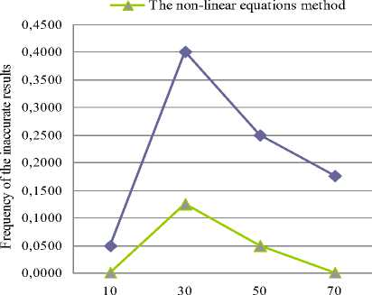
Fig. 1 shows inaccurate results comparison between the non-linear method and the frequency method with fixed graph density. Fig. 2 shows the same comparison but with fixed number of vertices.

The frequency method

The non-linear equations method

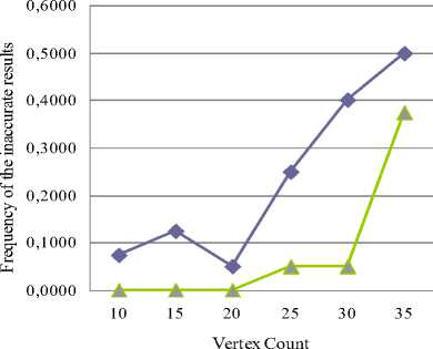
Fig.1. The inaccurate results comparison between the non-linear equations method and the frequency method with fixed density of 0.5

The frequency method

Graph Density, %

Fig.2. The inaccurate results comparison between the non-linear equations method and the frequency method with fixed number of vertices of 25

The frequency method is one of the most popular methods today. It has a time complexity of O (mn2) (where m is a number of edges, n is a number of vertices of a given graph) and in most cases the very low frequency of the inaccurate results. That’s why we are paying close attention to comparison between our nonlinear equations method and the frequency method.

To determine time complexity of the non-linear equations method we need also to analyze the number of operations that is required by the algorithm. The time complexity of the algorithm quantifies the amount of machine instructions it will execute as a function of the size of its input. Fig. 3 shows comparison of the number of operations with fixed graph density. Accordingly, Fig. 4 depicts such comparison with fixed number of vertices.

я

89 z

45000,0000

40000,0000

35000,0000

30000,0000

25000,0000

20000,0000

15000,0000

10000,0000

5000,0000

0,0000

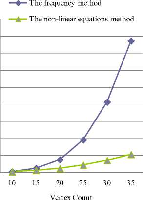
Fig.3. The number of operations comparison between the non-linear equations method and the frequency method with fixed density of 0.5

—♦— The frequency method

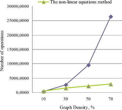
Fig.4. The number of operations comparison between the non-linear equations method and the frequency method with fixed number of vertices of 25

According to the results the non-linear equations method is much less dependent on a graph topology. While the value of the average degree gradually increases, the frequency of the inaccurate results (fig. 1 and fig. 2) of our method remains stable in comparison with the frequency method. Hence, the emulation experiment data prove that the non-linear equations method has an optimized approximation factor and, therefore, a relative error has a very low value even when using large-scale graphs. As shown in fig. 3 and fig. 4, the number of operations of the non-linear equations method is increased much slowly in comparison with the frequency method.

The difference between the methods is much apparent when the graph’s parameters are increased up to large values. Obviously, the non-linear equations method is much more effective and faster than its counterpart.

It worth noting that we ensure tests reliability by using a wide range of problem instances with different configurations. By means of our software package we generated different graph models such as the Erdős– Rényi model [15] and scale-free networks [17]. The Erdős–Rényi model is typically denoted as G(n, p), where n is a number of vertices of a given graph and p is a probability of an edge inclusion that is independent of the other edges. In other words, in such model each edge exists with the same probability. At the same time each vertex has the binomial distribution of the degree (the number of neighbors). Sometimes the number of vertices n tends to infinity during the analysis. However, in practice we must consider exact graph configurations. In this model the average degree is defined as np. So with the small value of p it is obvious that not every edge is connected.

The Erdős–Rényi model is well-suited for arbitrary degree distributions. For many realistic topologies (such as social networks, citation services etc.) it is worth taking into consideration the Barabási–Albert model that is used for generating scale-free networks. In this model degree distribution follows a power law that is defined as P(k) ~ k-λ , where k represents number of connections in a graph and λ is an optimization network parameter whose value lies in the range (2, 3) depending on particular graph instance. This model is often used for security reasons as the random removal of a large amount of vertices has a little impact on the overall connectedness of a graph.

According to the obtained data from the program the proposed algorithm runs in a polynomial time and outputs a solution that is close to the exact one. In particular, its approximation   ratio   is defined in the range

(( 2 - Θ 1   ), ( 2 - Θ 1     )) for the Barabási– k-λ           Vk-λ+1

Albert model and it stays stably (2 - Θ ¹   ) for the

Vlog np

Erdős–Rényi model.

In recent years the study of approximation technique has achieved great success. However, in many cases algorithms are optimized just for graphs with specific properties. In our work we propose method that can be used with different network topologies and with various nodes density. It can be even applied in the distributed environment taking into account high level of parallelization of instructions being involved in computation process.

Regarding the frequency method, it gives the best results only with the sparse graph instances. This method can still be used to minimize time for scheduling in heterogeneous systems even with the high scheduling activity, provided that the system nodes have small or medium connectedness. This will ensure minimal task downtime in a system and uniform resource loading.

One of the main characteristics of any theoretical methods is a practical application. The real-time environment often imposes such constraints that cannot be satisfied. The described method can be used in many practical real-time applications taking into account its improved performance and optimization for the dense graphs. Implementing that method in distributed systems and multi-core infrastructure can still increase the performance.

Future research will be directed to large-scale parallelization of the presented algorithm and investigation of solving similar problems.

• V.    Conclusion

A large number of science and technology problems are proved to be NP-hard problems. The main idea behind solving NP-hard problem is to find approximation solution. This paper considers an effective approximation algorithm with guaranteed predictions, which, according to experiment results, has an improved approximation factor.

We performed 50 different tests. According to our analysis, the non-linear equations method is much more efficient in comparison with one of the most currently fast and accurate algorithms. If the value of average degree gradually increases, other algorithms will have a great disadvantage in many aspects.