The scale invariant vacuum paradigm: main results plus the current BBNS progress

A. Motivation

The paper is a summary of the current main results within the Scale Invariant Vacuum (SIV) paradigm as related to the Weyl Integrable Geometry (WIG) as an extension to the standard Einstein General Relativity (EGR) as of Summer 2023. As such, it is a reflection of the corresponding online conference presentation during the XXIII International Meeting Physical Interpretations of Relativity Theory at the Bauman Moscow State Technical University, Moscow, 2023 (PIRT’23).

• ¹ E-mail: Vesselin at MailAPS.org

• ² E-mail: Andre.Maeder at UniGe.ch

  so to help the intellectually curious reader gain some understanding as to where the paradigm has been tested and what is the success level of the inquiry. As such, the paper follows closely our previous 2022 paper [6] that was based on a talk presented at the conference Alternative Gravities and Fundamental Cosmology, at the University of Szczecin, Poland in September 2021. Our initial presentation and its conference contribution were covering, back then, only four main results: comparing the scale factor a(t) within ACDM and SIV [13], the growth of the density fluctuations within the SIV [3], the application to scale-invariant dynamics of galaxies [4], and inflation of the early-universe within the SIV theory [2]. Back then, our article layout was aiming for focusing on each of these four main results via highlighting its most relevant figure or equation. As a result each topic was covered via one to two pages text preceded by short and concise description of the mathematical framework.

Here, we add one more sections related to the recent developments in the application of SIV paradigm since our previous summary paper in 2022 [6], it is our latest study of the Big-Bang Nucleosynthesis (BBNS) within the SIV Paradigm [5] that has been reported for a first time during PRIT’23 conference [7].

After a general introduction on the problem of scale invariance and physical reality, along with the similarities and differences of Einstein General Relativity and Weyl Integrable Geometry, we only highlight the mathematical framework as pertained to Weyl Integrable Geometry, Dirac Co-Calculus, and reparametrization invariance|. Rather than re-deriving the weak-field SIV results for the equations of motion, we have decided to use the idea of reparametrization invariance [8] to illustrate the corresponding equations of motion. The relevant discussion on reparametrization invariance is in the section on the Consequences of Going beyond Einstein’s General Relativity. This section precedes the brief review of the necessary results about the Scale Invariant Cosmology idea needed in the section on Comparisons and Applications, where we highlight the main results related to inflation within the SIV [2], the growth of the density fluctuations [3], and the application of the SIV to scale-invariant dynamics of galaxies, MOND, dark matter, and the dwarf spheroidals [4]. The results section of the paper concludes with the most recent results on the BBNS light-elements’ abundances within the SIV [5]. We end the paper with a section containing the Conclusions and Outlook for future research directions.

• A.1. Scale Invariance and Physical Reality

The presence of a scale is related to the existence of physical connection and causality. The corresponding relationships are formulated as physical laws dressed in mathematical expressions. The laws of physics (numerical factors in the formulae) change upon change of scale, but maintain a forminvariance. As a result, using consistent units is paramount in physics and leads to powerful dimensional estimates of the order of magnitude of physical quantities based on a simple dimensional analysis. The underlined scale is closely related to the presence of material content, which reflects the energy scale involved.

However, in the absence of matter, a scale is not easy to define. Therefore, an empty universe would be expected to be scale invariant! Absence of scale is confirmed by the scale invariance of the Maxwell equations in vacuum (no charges and no currents—the sources of the electromagnetic fields). The field equations of general relativity are scale invariant for empty space with zero cosmological constant. What amount of matter is sufficient to kill scale invariance is still an open question. Such a question is particularly relevant to cosmology and the evolution of the universe.

A.2. Einstein General Relativity (EGR) and Weyl Integrable Geometry (WIG)

Einstein’s General Relativity (EGR) is based on the premise of a torsion-free covariant connection that is metric-compatible and guarantees the preservation of the length of vectors along geodesics (8 U疗II = 0). The theory has been successfully tested at various scales, starting from local Earth laboratories, the Solar system, on galactic scales via light-bending effects, and even on an extragalactic level via the observation of gravitational waves. The EGR is also the foundation for modern cosmology and astrophysics. However, at galactic and cosmic scales, some new and mysterious phenomena have appeared. The explanations for these phenomena are often attributed to unknown matter particles or fields that are yet to be detected in our laboratories—dark matter and dark energy.

As no new particles or fields have been detected in the Earth labs for more than twenty years, it seems reasonable to revisit some old ideas that have been proposed as a modification of the EGR. In 1918, Weyl proposed and extension by adding local gauge (scale) invariance [9]. Other approaches were more radical by adding extra dimensions, such as Kaluza?Klein unification theory. Then, via Jordan conformal equivalence, one comes back to the usual 4D spacetime as pro jective relativity theory, but with at least one additional scalar field. Such theories are also known as Jordan?Brans?Dicke scalartensor gravitation theories [10, 11]. In most such theories, there is a major drawback—a varying Newton constant G. As no such variations have been observed, we prefer to view Newton’s gravitational constant G as constant despite the experimental issues on its measurements [12].

In the light of the above discussion one may naturally ask: could the mysterious (dark) phenomena be artifacts of non-zero 8 ||才|| , but often negligible; thus, almost zero value (8 ||才|| ^ 0), which could accumulate over cosmic distances and fool us that the observed phenomena may be due to dark matter and/or dark energy? An idea of extension of EGR was proposed by Weyl as soon as the General Relativity (GR) was proposed by Einstein. Weyl proposed an extension to GR by adding local gauge (scale) invariance that has the consequence that lengths may not be preserved upon parallel transport. However, it was quickly argued that such a model will result in a path dependent phenomenon and, thus, contradicting observations. A remedy was later found to this objection by introducing Weyl Integrable Geometry (WIG), where the lengths of vectors are conserved only along closed paths (ф 8 |才|| = 0). Such formulation of the Weyl’s original idea defeats the Einstein ob jection! Furthermore, given that all we observe about the distant universe are waves that reach us, the condition for Weyl Integrable Geometry is basically saying that the information that arrives to us via different paths is interfering constructively to build a consistent picture of the source.

One way to build a WIG model is to consider conformal transformation of the metric field g \ “ = 入 2 9 丛" and to apply it to various observational phenomena. As shown previously [1], the demand for homogeneous and isotropic space restricts the field A to depend only on the cosmic time and not on the space coordinates. The weak field limit of such a WIG model results in an extra acceleration in the equation of motion that is proportional to the velocity. This behavior is somewhat similar to the Jordan?Brans?Dicke scalar-tensor gravitation; however, the conformal factor A does not seems to be a typical scalar field as in the Jordan?Brans?Dicke theory [10, 11]. The Scale Invariant Vacuum (SIV) idea provides a way of finding out the specific functional form of A«) as applicable to LFRW cosmology and its WIG extension [1, 13].

We also find it important to point out that extra acceleration in the equations of motion, which is proportional to the velocity of a particle, could also be justified by requiring re-parametrization symmetry. Not implementing re-parametrization invariance in a model could lead to un-proper time parametrization [8] that seems to induce “fictitious forces” in the equations of motion similar to the forces derived in the weak field SIV regime. It is a puzzling observation that may help us understand nature better.

B. Mathematical Framework

The framework for the Scale Invariant Vacuum paradigm is based on the Weyl Integrable Geometry and Dirac co-calculus as mathematical tools for description of nature [9, 14].

The original Weyl Geometry uses a metric tensor field д^”, along with a “connexion” vector field Кд, and a scalar field A. In the Weyl Integrable Geometry, the “connexion” vector field 片丛 is not an independent, but it is derivable from the scalar field A via the defining expression:片丛=-дд ln(A). This form of the “connexion” vector field Кд guarantees its irrelevance, in the covariant derivatives, upon integration over closed paths. That is, § 冗其出c^ = 0. In other words,片丛“审丛 represents a closed 1-form; furthermore, it is an exact form since its definition implies K^dx^ = —d In A. Thus, the scalar function A plays a key role in the Weyl Integrable Geometry. Its physical meaning is related to the freedom of a local scale gauge, which provides a description upon scale change via local re-scaling 〃 т A(x)Z.

The covariant derivatives use the rules of the Dirac co-calculus [14] where tensors also have co-tensor powers based on the way they transform upon change of scale. For the metric tensor 呢“ this power is n = 2. This follows from the way the length of a line segment df with coordinates dx * is defined via the usual expression ds ² = g 呻 dx ^ dxJ That is, one has: 〃 т A(x)Z 台 ds^f = Adf 今 g *“ = A 2 g *^ . This leads to g *“ having the co-tensor power of n = — 2 in order to have the Kronecker S as scale invariant object (g *“ g "。 = S * ). That is, a co-tensor is of power n when, upon local scale change, it satisfies: 2 ' т A(x)Z : Y *" т A ⁿ Y *" , That is a scale-invariant EGR quantity denoted by primed quantity can be obtained from a WIG co-tensor of power n upon its multiplication by the A ⁿ factor.

In the Dirac co-calculus, this results in the appearance of the “connexion” vector field k * in the covariant derivatives of scalars, vectors, and tensors (see Table 1); where the usual Christoffel symbol Г *а is replaced by

• * г *。 = Г *。 + g * _a k " — g * K _tt — g ： k * .                            (B.1)

The corresponding equation of the geodesics within the WIG was first introduced in 1973 by [14] and in the weak-field limit of Weyl gauge change redivided in 1979 by [15] (u * = dx * /ds is the four-velocity):

d 〃 *

• u *" = 0 今—-- + Г * и u 。 + K " u u * = 0 .                     (B.2)

This geodesic equation has also been derived from reparametrization-invariant action in 1978 by [16] given by S / = / ^ ¹ S (ds) = / S (/ds) = / S @ 窮) d 丁 = 0.

Таблица 1.	Derivatives for co-tensors of power n defined via 匕^ т *Y“ when 厂 T A ( x ) Z.
	Co-Tensor Type Mathematical Expression
	co-scalar            S * * = d * S — nK * S,
	co-vector           A " * * = d * A " — * Г ：* 4 ： — ПК " Л * ,
	co-covector         Л "* = d * A " + * Г *： Л ： — nk " A * .

B.1. Consequences of Going beyond the EGR

Before we go into a specific examples, such as FLRW cosmology and weak-field limit, we would like to make few remarks. By using (B.1) in (B.2), one can see that the usual EGR equations of motion receive extra terms proportional to the four-velocity and its normalization:

• — --+ Г * u " u 。 = ( k • u)u * — (u • u ) k *                           (B.3)

ds 。

In the weak-field approximation within the SIV, one assumes an isotropic and homogeneous space for the derivation of the terms beyond the usual Newtonian equations [16]. As seen from (B.3), the result is a velocity dependent extra term к о ^ with k ° = — A/A and к = 0 due to the assumption of isotropic and homogeneous space. At this point, it is important to stress that the usual normalization for the four-velocity, u • u = ± 1 with sign related to the signature of the metric tensor g *" , is a special choice of s-parametrization—the proper-time parametrization 丁 .

Recently, similar k°不 term was derived as a consequence of non-reparametrization invariant mathematical modeling but without the need for a weak-field approximation. The effect is due to unproper time parametrization manifested as velocity dependent fictitious acceleration [8]. In this respect, the term k°不 is necessary for the restoration of the broken symmetry - the re-parametrization invariance of a process under study. To demonstrate this, one can apply an arbitrary time re-parametrization

A = dt/dr ; then, the first term on the LHS of (B.3) becomes:

^Adt 片)= ^A 2

dk

+ AAd.

(B.4)

By moving the term linear in the velocity to the RHS, dividing by A ² , and by using 片 (t) = - A/A, one obtains a /^o^like term on the RHS. If we were to do such manipulation in the absence of к₁0k on the RHS of (B.3), then the term will be generated, while if К was present then it will be transformed К T к + К.

Furthermore, unlike in SIV, where one can justify A(t) = t ° /t [13], for re-parametrization symmetry the time dependence of A(t) could be arbitrary. Finally, as discussed in [8], the extra term к ° 不 is not expected to be present when the time parametrization of the process is the proper time of the system. Thus, a term of the form к 不 can be viewed as restoration of the re-parametrization symmetry and an indication of un-proper time parametrization of a process under consideration.

• B.2.    Scale Invariant Cosmology

  The scale invariant cosmology equations were first introduced in 1973 by [14] and then re-derived in 1977 by [17]. The equations are based on the corresponding expressions of the Ricci tensor and the relevant extension of the Einstein equations. The conformal transformation (项“ = X 2 g ^_y ) of the metric tensor g ^" in the more general Weyl’s framework into Einstein’s framework, where the metric tensor is g\u , induces a simple relation between the Ricci tensor and scalar in the Weyl’s Integrable Geometry and the Einstein GR framework (using prime to denote Einstein GR framework ob jects):

冗 H" = R "" ^{— к} 因" ^{— к} "屮^— 2 ^к д ^к " ⁺ 2^д н" ^{к к} а ^{— д} н" ^к ； @     ^and R = R ⁺ 6^{K к} а ^— 6 ^к ； @ ■

By considering the Einstein equation R ^” — 2 g^R = S^GT ^" — Л g^ along with the above expressions, one gets:

R H"

g #

；"

R ’ —

^K H ； "

^K " ； H

^— 8^^GT H" - ^Л g #"

(B.5)

The relationship Л = А ² Ле of Л in WIG to the Einstein cosmological constant Ле in the EGR was present in the original form of the equations to provide explicit scale invariance. This relationship makes explicit the appearance of Ле as invariant scalar (in-scalar), as then one has Л g #" = А ² Ле g #" = Ле g #" .

The above equation (B.5) ia a generalization of the original Einstein GR equation. Thus, they have an even larger class of local gauge symmetries that need to be fixed by a gauge choice. In Dirac’s work, the gauge choice was based on the large numbers hypothesis. Here, we will discuss a different gauge choice - the SIV gauge.

The corresponding scale-invariant FLRW based cosmology equations within the WIG framework were first introduced in 1977 by [17]:

8 冗 Go

人 + 岂 ₊₂ ^+_-…

Q ² Q ² Aq A ²     3

. ck c^ J Q²    ,qA A²   .   、 2

and — 8 ^Gp = —2 + 2 —+2* +—2 +4 —^ — ^ 2 — Ле A . (B.6)

These equations clearly reproduce the standard FLRW equations in the limit A = const = 1. The scaling of Л was recently used to revisit the Cosmological Constant Problem within quantum cosmology [18]. The conclusion of [18] is that our universe is unusually large, given that the expected mean size of all universes, where Einstein GR holds, is expected to be of a Plank scale. In the study, A = const was a key assumption as the universes were expected to obey the Einstein GR equations. What the expected mean size of all universes would be if the condition A = const is relaxed, as for a WIG-universes ensemble, remains an open question.

• B.3.    The Scale Invariant Vacuum Gauge ( T = 0 and R = 0 )

The idea of the Scale Invariant Vacuum was introduced first in 2017 by [13]. It is based on the fact that, for Ricci flat ( 冗 厶“ =0) Einstein GR vacuum (厶“ =0), one obtains from (B.5) the following equation for the vacuum:

片 其； " + 左 " 屮 + 2 片 H 片 " - 2g 叩 00 + 9 h" 左 左 a = ^л 呢".

(B.7)

For homogeneous and isotropic WIG-space &X = 0; therefore, only 片0 = —A/A and its time derivative 百о =—片0 can be non-zero. As a corollary of (B.7), one can derive the following set of equations [13]:

.A ² A …一 ²_A       A A ²    / A  A ² л

³ 帀 =^л, ^{and 2}A - * =^л,  ^or A = ² 帀 , ^and  A - 帀 =з .           ⁽ B.8)

One could derive these equations by using the time and space components of the equations (B.7) or by looking at the relevant trace invariant along with the relationship 百 о = — к 0 . Any pair of these equations is sufficient to prove the other pair of equations.

Theorem 1. Using any one pair of two SIV Equations (B.8) along with Л = ^Ле one has ：

Л 石 =3 A 4 ， ^with 嘗 =0.

(B.9)

Corollary. The solution of the SIV equations is: A = 力 о /力， with 力 о = ， 3 / Л 石 and с = 1 for the speed of light.

Upon the use of the SIV gauge, first in 2017 by [13], one observes that the cosmological constant disappears from Equations (B.6):

8 冗 Go

k 勿 ² lA

酒 + a 2 + ² 否

and

— 8^Gp

k   c^ Q ² ，勿 A

F + 2—I—+ 4—-.

Q ²     Q Q ²     QA

(B.10)

• C. Comparisons and Applications

The predictions and outcomes of the SIV paradigm were confronted with observations in a series of papers by the current authors. Highlighting the main results and outcomes is the sub ject of current section.

C.1. Comparing the Scale Factor a ⑴ within A CDM and SIV

Upon arriving at the SIV cosmology Equations (B.10), along with the gauge fixing (B.9), which implies A = 力°〃 with 力 о indicating the current age of the universe since the Big-Bang ( q = 0 at 力由 < 力 о ), the implications for cosmology were first discussed by [13] and later reviewed by [19]. The most important point in comparing ЛCDM and SIV cosmology models is the existence of SIV cosmology with slightly different parameters but almost the same curve for the standard scale parameter q ( ^ ) when the time scale is set so that 力 о = 1 now [13, 19]. As seen in Figure 1, the difference between the ЛCDM and SIV models declines for increasing matter densities. Furthermore, for any ЛCDM curve at some Q ^ there is a matching SIV curve at some Q _m <  Q ^ . Thus, SIV needs less total matter to produce the same scale-factor evolution.

C.2. Application to Scale-Invariant Dynamics of Galaxies

The next important application of the scale-invariance at cosmic scales is the derivation of a universal expression for the Radial Acceleration Relation (RAR) of g obs and g bar . That is, the relation

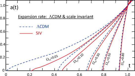
Рис. 1. Expansion rates a(t) as a function of time t in the flat ( 用 =0) ACDM and SIV models in the matter dominated era. The curves are labeled by the values of Q m .

between the observed gravitational acceleration g°bs = v2/r and the baryonic matter acceleration due to the standard Newtonian gravity 9n by [4]:

к 2    1 г. -------тт

9 = 9 n + £ + 2 ， 4 奴足 ² + к ,

(C.1)

where 9 = g °bs , g z = 9 bar . For 9 n 》 к ² : g т 9 n but for 9 n t 0 今 g т к ² is a constant.

As seen in Figure 2, MOND deviates significantly for the data on the Dwarf Spheroidals. This is well-known problem in MOND due to the need of two different interpolating functions, one in galaxies and one at cosmic scales. The SIV expression (C.1) resolves this issue via one universal parameter к ² related to the gravity at large distances [4]. Even more, one can actually show that MOND is a peculiar case of the SIV theory [20].

] 2- s m[ g go

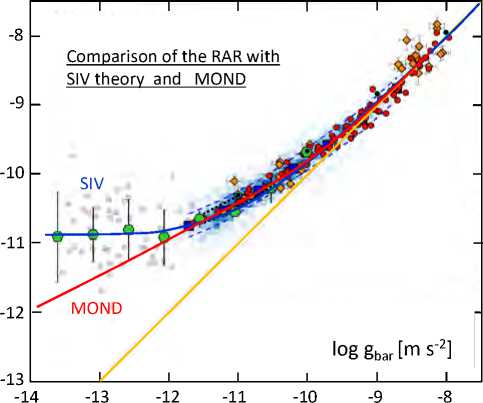
Рис. 2. Radial Acceleration Relation (RAR) for the galaxies studied by Lelli et al. (2017). Dwarf Spheroidals as binned data (big green hexagons), along with MOND (red curve), and SIV (blue curve) model predictions. The orange curve shows the 1:1-line for g °bs and g bar . Due to to the smallness of g °bs and g bar the application of the log function results in negative numbers; thus, the corresponding axes’ values are all negative.

The expression (C.1) follows from the Weak Field Approximation (WFA) of the SIV upon utilization of the Dirac co-calculus in the derivation of the geodesic equation within the relevant WIG (B.2) (see

[4] for more details, as well as the original derivation in [15]):

仇勿 = - 1, 9 00

1 + 2Ф/с 2 今「 00

1 2g 00

2 дМ

1 дФ с2 дхі

今

医标_GM7     dM dt2 г2 г +'° '必.

(C.2)

where ， е 1,2, 3, while the potential Ф = GM/r is scale invariant.

By considering the scale-invariant ratio of the correction term ' o (t) 不 to the usual Newtonian term

Н О (Н J obs ) ^{1 / 2}      9 obs -9 bar

£     g bar            g bar

in (C.2), one has: т = 唱客 = 知务²

Then, by utilizing an explicit scale

5/VJ         彳 Lj VI invariance for cancelingthe proportionality factor: ( ^bg-gba『(g°b^)1 = ( fob^ )1/2 (仁卜 by setting g = 9obs,2, 9n = 9bar,2, and by collecting all the system-1 terms in к =日⑴，then one arrives at (C.1) by solving for g in 訖 —1 = k(i)fg/- and keeping the bigger root (the positive sign in 士,...

factor).

C.3. Growth of the Density Fluctuations within the SIV

Another interesting result was the possibility of a fast growth of the density fluctuations within the SIV [3]. This study accordingly modifies the relevant equations such as the continuity equation, Poisson equation, and Euler equation within the SIV framework. Here, we outline the main equations and the relevant results.

By using the notation 呂 =' ° = — A/A = 1/t, the corresponding Continuity, Poisson, and Euler equations are:

用 + V • (p/) = ' [ p + r • V p ] , V ² Ф = Л Ф = 4 冗 G. \^ = 留 + (不 • V )不 = —V Ф — -Vp + '不.

For a density perturbation q ( x, t) = 0 b (t)(1 + 8(/,t)) the above equations result in:

$ + V • / = '/ • V b = n'(t)5,     V ²W = 4^Ga 2 Q b S,   / + 2Н/ + (/ • V )/ = —^^ + '(t)/. (C.3)

Q ²

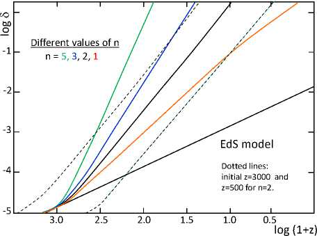
Рис. 3. The growth of density fluctuations for different values of parameter n (the gradient of the density distribution in the nascent cluster), for an initial value 8 = 10 -5 at z = 1376 and Q m = 0.10. The initial slopes are those of the EdS models. The two light broken curves show models with initial (z + 1) = 3000 and 500, with same Q m = 0.10 and n = 2. These dashed lines are to be compared to the black continuous line of the n = 2 model. All the three lines for n = 2 are very similar and nearly parallel. Due to to the smallness of 8 the application of the log function results in negative numbers; resulting in negative vertical axis.

The final result $ + (2" — (1 + 几)')$ = 4^G^b$ + 2w(H — ')$ recovers the standard equation in the limit of ' T 0. The simplifying assumption / • V$(x)=几$(x) in (C.3) introduces the parameter 几 that measures the perturbation type (shape). For example, a spherically symmetric perturbation would have n = 2. As seen in Figure 3, perturbations for various values of n are resulting in faster growth of the density fluctuations within the SIV than in the Einstein–de Sitter model, even at relatively law matter densities. Furthermore, the overall slope is independent of the choice of recombination epoch 入)The behavior for different Qm is also very interesting, and is shown and discussed in detail by [3].

C.4. Big-Bang Nucleosynthesis within the Scale Invariant Vacuum Paradigm

The SIV paradigm has been recently applied to the Big-Bang Nucleosynthesis using the known analytic expressions for the expansion factor q and the plasma temperature T as functions of the SIV time 丁 since the Big-Bang when 。 ( 丁 = 0) = 0 [5]. The results have been compared to the standard BBNS as calculated via the PRIMAT code [21]. Potential SIV-guided deviations from the local statistical equilibrium were also explored in ref. [5]. Overall, it was found that smaller than usual baryon and non-zero dark matter content, by a factor of three to five times reduction, result in compatible to the standard light elements abundances (Table 2).

The SIV analytic expressions for a(T ) and 丁 (T ) were utilized to study the BBNS within the SIV paradigm [5, 22]. The functional behavior is very similar to the standard model within PRIMAT except during the very early universe where electron-positron annihilation and neutrino processes affect the a(T ) function (see Table I and Fig. 2 in ref. [5]). The distortion due to these effects encoded in the function S(T) could be incorporated by considering the SIV paradigm as a background state of the universe where these processes could take place. It has been demonstrated that incorporation of the S(T ) within the SIV paradigm results in a compatible outcome with the standard BBNS see the last two columns of Table 2; furthermore, if one is to fit the observational data the result is A ^ 1 for the SIV parameter A (see last column of Table 2 with A = FRF ^ 1). However, a pure SIV treatment (the middle three columns) results in Q ^ ^ 1% and less total matter, either around Q _m ^ 23% when all the A-scaling connections are utilized (see Table 2 column 6), or around Q _m ^ 6% without any A-scaling factors (see column 5 of Table 2). The need to have A close to 1 is not an indicator of dark matter content but indicates the goodness of the standard PRIMAT results that allows only for A close to 1 as an augmentation, as such this leads to a light but important improvement in D/H as seen when comparing columns three with eight and nine.

The SIV paradigm suggests specific modifications to the reaction rates, as well as the functional temperature dependences of these rates, that need to be implemented to have consistence between the Einstein GR frame and the WIG (SIV) frame. In particular, the non-in-scalar factor T ° in the reverse reactions rates may be affected the most due to the SIV effects. As shown in [5], the specific dependences studied, within the assumptions made within the SIV model, resulted in three times less baryon matter, usually around Q ^ ^ 1.6% and less total matter - around Q _m ^ 6%. The lower baryon matter content leads to also a lower photon to baryon ratio 〃 io ^ 2 within the SIV, which is three tines less that the standard value of тую = 6.09. The overall results indicated insensitivity to the specific A-scaling dependence of the mT-factor in the reverse reaction expressions within T ° terms. Thus, one may have to explore further the SIV-guided A-scaling relations as done for the last column in Table 2, however, this would require the utilization of the numerical methods used by PRIMAT and as such will take us away from the SIV-analytic expressions explored that provided a simple model for understanding the BBNS within the SIV paradigm. Furthermore, it will take us further away from the accepted local statistical equilibrium and may require the application of the reparametrization paradigm that seems to result in SIV like equations but does not impose a specific form for A [8].

C.5. SIV and the Inflation of the Early Universe

The latest published result within the SIV paradigm is the presence of inflation stage at the very early universe 力 ^ 0 with a natural exit from inflation in a later time 力 exit with value related to the parameters of the inflationary potential [2]. The main steps towards these results are outlined below.

Element	Obs.	PRMT	aSW	fit	fit*	a/A	fit*	fit
H	0.755	0.753	0.805	0.755	0.849	0.75	0.753	0.755
Yp =4! He	0.245	0.247	0.195	0.245	0.151	0.25	0.247	0.245
D/H X 10 5	2.53	2.43	0.743	2.52	2.52	1.49	2.52	2.53
3 He/H X 10 5	1.1	1.04	0.745	1.05	0.825	0.884	1.05	1.04
7 Li/H X 10 10	1.58	5.56	11.9	5.24	6.97	9.65	5.31	5.42
N eff	3.01	3.01	3.01	3.01	3.01	3.01	3.01	3.01
〃 10	6.09	6.14	6.14	1.99	0.77	1.99	5.57	5.56
FRF	1	1	1	1	1.63	1	1	1.02
mTˇ	1	1	1	1	0.78	1	1	0.99
Q/Tˇ	1	1	1	1	1.28	1	1	1.01
Q b [%]	4.9	4.9	4.9	1.6	0.6	1.6	4.4	4.4
Q m [%]	31	31	31	5.9	23	5.9	86	95
V x f	N/A	6.84	34.9	6.11	14.8	21.9	6.2	6.4

Таблица 2. The observational uncertainties are 1.6% for У р , 1.2% for D/H, 18% for T/H, and 19% for Li/H. FRF is the forwards rescale factor for all reactions, while mT ^ˇ and Q/T ^ˇ are the corresponding rescale factors in the revers reaction formula based on the local thermodynamical equilibrium. The SIV ^-dependences are used when these factors are different from 1; that is, in the sixth and ninth columns where FRF=A, mT= A ^-1 / ² , and Q/T= A +^1/2 . The columns denoted by fit contain the results for perfect fit on Q ^ and Q _m to 4 He and D/H, while fit* is the best possible fit on Q & and Q _m to the 4 He and D/H observations for the model considered as indicated in the columns four and seven. The last three columns are usual PRIMAT runs with modified a ( T ) such that 值 /A = a siv /S ^1/3 , where 值 is the PRIMAT’s a ( T ) for the decoupled neutrinos case. Column seven is actually a siv /S ^1/3 , but it is denoted by a/A to remind us about the relationship a ' = aA; the run is based on Q b and Q _m from column five. The smaller values of 力 0 are due to smaller % 2 Q b , as seen by noticing that ^ 10 /Q b is always ^ 1.25.

If we go back to the first of the general scale-invariant cosmology Equations (B.6), we can identify a vacuum energy density expression that relates the Einstein cosmological constant with the energy density as expressed in terms of 片 = — A/A by using the SIV result (B.9). The corresponding vacuum energy density 夕， with C = 3 / (4t tG ) , is then:

^Л       2 ‘   、 2 ^Л 石       ^{3 A} 2 ^C 2

^P =菰 =^A 0 = ^A =贰* = 也 .

This provides a natural connection to inflation within the SIV via ^ = — A/A or ^ к ln«). The equations for the energy density, pressure, and Weinberg’s condition for inflation within the standard inflation [23, 24, 25, 26] are:

P p

20 ² ± V3, | 玄 nfl I« 碗 fl .                          (C.4)

If we make the identification between the standard inflation above with the fields within the SIV (using C = 3 / (4t tG ) ):

v> = — A/A, 0 о V C^, V о CU 侬) ，。 侬) =ge "吵 .               ( C.5)

Here, U(3) is the inflation potential with strength g and field “coupling” 〃 . One can evaluate the

Weinberg’s condition for inflation (C.4) within the SIV framework [2], and the result is:

"=й^) 厂"² « Uof^2, andt 京 ' 0 = 1.

From this expression, one can see that there is a graceful exit from inflation at the later time:

I ng texit ^ у 3F+^

with n = — 〃 — 2 >  0 ,

(C.6)

(C.7)

when the Weinberg’s condition for inflation (C.4) is not satisfied anymore. For more details, we refer the reader to the derivation of the equation (C.6) presented in our previous papers [1, 2].

D. Conclusions and Outlook

From the highlighted results in the previous section on various comparisons and potential applications, we see that the SIV cosmology is a viable alternative to ACDM. In particular, within the SIV gauge (B.10) the cosmological constant disappears. There are diminishing differences in the values of the scale factor q(" within ACDM and SIV at higher densities as emphasized in the discussion of (Figire 1) [13, 19]. Furthermore, the SIV also shows consistency for H o and the age of the universe, and the m-z diagram is well satisfied—see [19] for details.

Furthermore, the SIV provides the correct RAR for dwarf spheroidals (Figure 2) while MOND is failing, and dark matter cannot account for the phenomenon [4]. Therefore, it seems that within the SIV, dark matter is not needed to seed the growth of structure in the universe, as there is a fast enough growth of the density fluctuations as seen in (Figure 3) and discussed in more detail by [3].

As to the BBNS within the SIV, our main conclusion is that the SIV paradigm provides a concurrent model of the BBNS that is compatible to the description of ⁴ He, D/H, T/H, and ⁷ Li/H achieved in the standard BBNS. It suffers of the same ⁷ Li problem as in the standard BBNS but also suggests a possible SIV-guided departure from local statistical equilibrium which could be a fruitful direction to be explored towards the resolution of the ⁷ Li problem.

In our study on the inflation within the SIV cosmology [2], we have identified a connection of the scale factor A, and its rate of change, with the inflation field ^ т 夕， ^ = — A/A (C.5). As seen from (C.6), inflation of the very-very early universe (t ^ 0) is natural, and SIV predicts a graceful exit from inflation (see (C.7))!

Some of the obvious future research directions are related to the primordial nucleosynthesis, where preliminary results show a satisfactory comparison between SIV and observations [5, 22]. The recent success of the R-MOND in the description of the CMB [27], after the initial hope and concerns [28], is very stimulating and demands testing SIV cosmology against the MOND and ACDM successes in the description of the CMB, the Baryonic Acoustic Oscillations, etc.

Another important direction is the need to understand the physical meaning and interpretation of the conformal factor A. As we pointed out in the Motivation Section, a general conformal factor A ( t ) seems to be linked to Jordan?Brans?Dicke scalar-tensor theory that leads to a varying Newton’s constant G, which has not been found in nature. Furthermore, a spacial dependence of A ( t ) opens the door to local field excitations that should manifest as some type of fundamental scalar particles. The Higgs boson is such a particle, but a connection to Jordan?Brans?Dicke theory seems a far fetched idea. On the other hand, the assumption of isotropy and homogeneity of space forces A(t) to depend only on time, which is not in any sense similar to the usual fundamental fields we are familiar with.

In this respect, other less obvious research directions are related to the exploration of SIV within the solar system due to the high-accuracy data available, or exploring further and in more detail the possible connection of SIV with the re-parametrization invariance. For example, it is already known by [8] that un-proper time parametrization can lead to a SIV-like equation of motion (B.3) and the relevant weak-field version (C.2).

Acknowledgments

A.M. expresses his gratitude to his wife for her patience and support. V.G. is extremely grateful to his wife and daughters for their understanding and family support during the various stages of the research presented. This research did not receive any specific grant from funding agencies in the public, commercial, or not-for-profit sectors. V.G. is grateful to the organizers of the PRIT’23 conference for their kind accommodations needed for V.G. to be able to present online this research results.