The SEIQR–V model: on a more accurate analytical characterization of malicious threat defense

Author: ChukwuNonso H. Nwokoye, Ikechukwu I. Umeh
Journal: International Journal of Information Technology and Computer Science @ijitcs
Article in issue: 12 Vol. 9, 2017.
Free access
Epidemic models have been used in recent times to model the dynamics of malicious codes in wireless sensor network (WSN). This is due to its open nature which provides an easy target for malware attacks aimed at disrupting the activities of the network or at worse, causing total failure of the network. The Susceptible-Exposed-Infectious-Quarantined-Recovered–Susceptible with a Vaccination compartment (SEIQR-V) model by Mishra and Tyagi is one of such models that characterize worm dynamics in WSN. However, a critical analysis of this model and WSN epidemic literature shows that it is absent essential factors such as communication range and distribution density. Therefore, we modify the SEIQR-V model to include these factors and to generate better reproduction ratios for the introduction of an infectious sensor into a susceptible sensor population. The symbolic solutions of the equilibriums were derived for two topological expressions culled from WSN literature. A suitable numerical method was used to solve, simulate and validate the modified model. Simulation results show the effect of our modifications.
Epidemic model, Wireless sensor network, Worm, Communication range, Distribution density
Short address: https://sciup.org/15016216
IDR: 15016216 | DOI: 10.5815/ijitcs.2017.12.04
Text of the scientific article The SEIQR–V model: on a more accurate analytical characterization of malicious threat defense
Published Online December 2017 in MECS DOI: 10.5815/ijitcs.2017.12.04
Wireless sensor network (WSN) is a network of sensors that cooperatively sense and perhaps control the environment, in such a manner that it allows person/computer-environment interactions [1]. Characteristically, WSN comprises of a large number of sensor nodes deployed randomly inside of or near the monitoring area (sensor field), form networks through self-organization [2]. The collected data are communicated to neighboring nodes through a multi-hop architecture. During the process of data transmission, monitored/collected data may be handled by multiple nodes to get to a gateway node through multi-hop routing. Basically these deployed sensors are tiny, miniature but low-battery-powered devices wherein functions such as sensing (and data collection), processing (or determining routing paths etc) and communication (sending the collected data to a chosen destination) are integrated. As a result a cross-layer design strategy that jointly considers signal or date processing, medium access control and communication protocols emerges. As Nwokoye et al. [3] puts it, “the applications of sensor networks are evident in the military (for monitoring forces/equipments, battlefield surveillance, reconnaissance, targeting, battle damage evaluation); in the environment (for biocomplexity mapping, precision agriculture, fire and flood detection etc) and in the home. Its use extends also to health applications (for telemonitoring of data, tracking/monitoring of doctors/patients and drug administration) and other commercial applications.”
WSN is fraught with several challenges; they include limited battery life, faster bandwidth utilization, transmission range, uncertainties in topology control and deployment. Other challenges of the WSN include “simplicity, coverage, connectivity, scalability, robustness, fault-tolerance, security, efficient use of energy” [4]. Beside its deployment in un-trusted, unguarded and unfriendly terrain, there is the issue of communication which is done in an open air medium, making the WSN an attractive target for malicious attacks that are aimed at disrupting the normal operation of the network. With the prevalence of cyberspace attacks such sinkhole, sybil, wormhole and hello flood and the emergence of malwares such as cabir and mabir (that propagate without human intervention), there became an urgent need to provide a robust defense structure for industries/organization that use the WSN for daily meaningful work. To do the needful, network security researchers employ the classic epidemic models, but as it’s widely known, the strength of a model is predicated on the extent to which it can aid better understanding and abstraction of the phenomena in question. In other words,
(depending on the analyst’s aim) a model with limited abstraction/characterization of a phenomenon gives limited results/outcomes.
-
II. Related Works
Researchers in the field of network security have discovered certain sameness in connectivity realities between biological viruses in human populations and malware equivalents in telecommunication/technological networks, and this has motivated the application of epidemic theory for defense against possible epidemic in ICT infrastructures. The Susceptible-Infected-Recovered (SIR) by Kermack and Mckendrick [5-7] initiated the investigation of infectious results of a susceptible network population. Thereafter, several modification ensued; involving factors that seek to characterize emerging/challenging issues in computer networks, peer-to-peer networks and wireless sensor and adhoc networks. Unlike the SIR model, the Susceptible-Infected (SI) model does not involve the recovery/removed class in its analyses, and so is the Susceptible-Infected-Susceptible (SIS) model. But while the SIS assumes a transfer back to the susceptible class, the SI does not.
In a bid to model the topological implications of several omindirectionally-equipped-sensors placed on a grid, Khayam and Radha [8] proposed the topology-aware worm propagation model (TWPM). Here, a sensor is surrounded and may infect its eight neighboring sensors and when infective can spread the infection to its neighbors. Their model involved parameters for the physical, media access control (MAC), network and transport layer protocols.
Using TWPM, Khayam and Radha [9] employed signal processing strategy in order to characterize the time/space-related dynamics of malware propagation. More so, through parameterized equations they integrated the features of data and network protocols. Their work simplified the frequency domain and performed simulation experiments that demonstrated the TWPM’s effectiveness and accuracy in modeling worm propagation in sensor networks.
To curb the potential spread of virus that causes node compromise, De, Liu, and Das [10] investigated the use of random graphs structured in accordance to real world network parameters. This is to generate insights that allow network managers to curb network epidemics. Their model also proposed the pairwise key schemes employs the predistribution strategy instead of the online key management schemes. This is due to serious resource deficiencies and the constrained network bandwidth of the wireless sensor networks. De, Liu, and Das [11] studied the vulnerability of popular multi-hop broadcast protocols in terms of reachability and speed. Their proposed model parameterized the communication patterns of Trickle, Deluge and MNP. Assuming that broadcast protocol propagation originates from a single node and in a ripple-like manner spreads to other nodes with the passage of time, De, Liu, and Das [12] modeled two node deployment patterns, namely: uniform random and group-based deployment.
Tang and Mark [13] added a maintenance functionality to the basic SIR model in order to characterize possible spread and defense of a viral infection in the wireless sensor network. At the maintenance state, the program for system maintenance (which involves very effective antivirus software) is triggered automatically. Their studies showed that changes in the topology of the network as well as energy consumption can affect propagation dynamics of the malware.
The fact that sensor nodes can become dead due to the depletion of their minimal battery power motivated Wang and Li [14] to propose the nonlinear iSIR model which describes malware patterns in large sensor networks. Using Vinsim 5.0 – a system dynamics software, they simulated three hypothetical cases of the random features of state transition in WSN.
Due to the absence of a popular policy for elongating the life time of sensors in [14], Wang, Li and Li [15] proposed the EiSIRS model which considers the sleep and work interleaving schedule for nodes. This model unlike the model in [14] does not assume that the sensors work all the time i.e. the susceptible, the infectious and the recovered nodes can be in either sleeping or working mode.
Tang [16] applied the maintenance mechanism using the SI epidemic model; therein sensors can be made free of any infection before they go to sleep without extra overhead cost on the hardware and the signaling mechanism.
Aside sensor temporary recovery, Mishra and Keshri [17] developed the Susceptible-Exposed-Infective-Recovered-Susceptible model with a vaccination (SEIR-V) model which assumes that sensor nodes can be inoculated against future infection or be exposed to infection wherein transmission speed becomes slow. Their work generated the reproduction ratio that suggests the number of secondary infections arising as a result of introducing an infectious sensor into a susceptible population.
Considering topology or distribution of sensor nodes, Wang and Yang [18] investigated the impact of medium access control (MAC) on virus propagation. Like Tang and Mark [13], viral behavior is sensitive to changes in topology and transmission range i.e. the increase of these factors increased the number of infectious nodes in the network.
Mishra, Srivastava, and Mishra [19] proposed the Susceptible - Infected - Quarantine - Recovered – Susceptible (SIQRS). This model did not consider the latent (or exposed) stage of worms wherein sensors may show symptoms such as slow transmission speed. In addition the vaccination compartment wasn’t included in the model.
Mishra and Tyagi [20] proposed the Susceptible-Exposed–Infectious–Quarantine–Recovered with Vaccination (SEIQR-V) epidemic model to describe worm dynamics in WSN. This model modified the SEIR-V model in Mishra and Keshri [17] by adding a quarantining (isolation) compartment.
Zhang and Si [21] choose delay as a bifurcation parameter in order to investigate the existence of Hopf bifurcation in the SEIR-V epidemic model by [17]. Therein they investigated the attributes of the Hopf bifurcation using the normal form method and the center manifold theorem. It was discovered an unwelcomed state in WSN wherein the prevalence of worms transits from positive equilibrium to a limit cycle.
While Tang and Mark [13], Wang and Yang [18] used a certain expression for uniform random distribution, Feng et al. [22] employed the expression used by Wang and Li [14] to evaluate the impact of communication radius, energy consumption and node distribution density in WSN. In their work the jacobian method was used to investigate the local stability while the lyapunov theorem was used to study the global stability. However, their work didn’t consider the latent stage of worms, sensor isolation and sensor vaccination.
Nwokoye, Ozoegwu and Ejiofor [23] explored the possibilities of determining the health status of an immigrant sensor using the Q-SEIRV epidemic model.
From the reviewed works herein, Tang and Mark [13], Mishra and Keshri [17], Mishra, Srivastava, and Mishra [19], Mishra and Tyagi [20], Feng et al. [22] generated reproduction ratios for the introduction of a single infective sensor in a fully susceptible population. On the other hand, the following works did not investigate the stability of equilibriums existent in a wireless sensor network; they include Khayam and Radha [8], Khayam and Radha [9], De, Liu, and Das [10], De, Liu, and Das [11], De, Liu, and Das [12], Tang and Mark [13], Wang and Li [14], Wang, Li and Li [15], Tang [16] and Wang and Yang [18].
Though Mishra and Tyagi [20] proposed the SEIQR-V epidemic model for WSN dynamics in a paper published in the International Journal of Information Technology and Computer Science; their characterization and analyses did not include any of the expressions for uniform random distribution noted above. The implication is that the reproduction number generated from their study may be strongly limited because of the absence of transmission range and distribution density.
However, from Nwokoye et al. [24], it is evident that the expression for range and density form part of the reproduction number. In this study, the SEIQR-V is modified to include the analysis for the impact of transmission range and density. The topological expressions described in Tang and Mark [13], Wang and Yang [18] and Feng et al. [22] and Wang and Li [14] will prove useful.
-
III. The Modified Seiqr-V Epidemic Model
Here, we modify the Susceptible-Exposed-Infectious-Quarantined-Recovered–Susceptible with a Vaccination compartment (SEIQR-V) model of Mishra & Tyagi [20]. In this study, we refer to the modification of the SEIQR-V model using the expression for uniform random distribution in [13,18] as Model 1. On the other hand, the modification of the SEIQR-V model with slightly different expression found in [14,22] will be referred to as Model 2. These expressions describe distribution density and range in WSNs; however, the latter involved the length of side ( L ) and this is absent in the former.
-
A. Model Assumptions
We characterize worm attack in wireless sensor network using the Susceptible–Exposed–Infectious– Quarantined–Recovered–Susceptible with a Vaccination compartment (SEIQR-V) model. For the sake of clarity, the model parameters used for characterizing the dynamics of worm propagation in wireless sensor networks are presented and described in Table 1.
Table 1. WSN Parameters and Their Meaning
|
Parameters |
Name |
Meaning |
|
a |
alpha |
Rate of transmission from the infectious compartment to the quarantined compartment |
|
77 |
eta |
Rate of transmission from the quarantined to the recovered compartment |
|
σ |
sigma |
Distribution density |
|
'0 |
r |
Transmission range |
|
ОЛТд |
- |
Effective contact with an infected node for transfer of infection for Model 1 |
|
L2 |
- |
Length of side |
|
ОЛТд2 / L2 \ |
- |
Effective contact with an infected node for transfer of infection for Model 2 |
|
A |
lambda |
Inclusion rate of nodes into the sensor network population |
|
p |
beta |
Infectivity contact rate |
|
T |
tau |
Death rate of nodes due to hardware or software failure |
|
d) |
omega |
Crashing rate due to attack of malicious objects (in this case worm) |
|
6 |
theta |
Rate at which exposed nodes become infectious |
|
V |
nu |
Rate of recovery |
|
Ф |
phi |
Rate at which recovered nodes become susceptible to infection |
|
p |
rho |
Rate of vaccination for susceptible sensor nodes |
|
xi |
Rate of transmission from the Vaccinated compartment to the Susceptible compartment |
The total population N(t) represents the nodes in the Wireless Sensor Network which is subdivided into Susceptible, Exposed, Infectious, Quarantined, Recovered, Vaccinated denoted by S(t), E(t), I(t), Q(t), R(t) and V(t). This implies that S (t) + E (t) + I (t) + Q (t) + R (t) + V (t) = N(t).
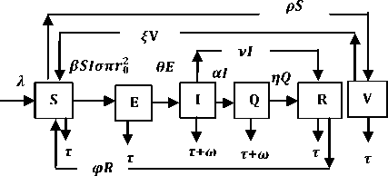
Fig.1. Schematic Diagram for the Flow of Worms in WSN
The schematic diagram for the dynamical transmission of worms in a WSN given our assumption is depicted in Fig. 1. The system of differential equation (1) is adapted from [20] but modified to capture distribution density and transmission range. The modified SEIQR-V model is represented using the following system of differential equations;
S = Л - PSIстяг02 - tS - pS + rR + fV
Ё = PSIстяг02 - (t + 6 )E
I = 6E - (t + ш + v + «)I (1)
Q = «I - (t + ti + p )Q
R = p Q + vI - (t + p )R
V = pS - (t + f)V equilibrium and the endemic equilibrium points i.e. S = 0; E = 0; I = 0; 5 = 0;Р = 0;У = 0. The worm-free equilibrium describes the absence of worms while the endemic equilibrium describes the presence of worms in the WSN using the formulated mathematical model. However, we observed that solutions at the worm-free equilibrium are the same for both models.
The solutions of equilibrium points are Worm-free equilibrium E0F = (S * ,E * ,I * ,Q *,R * , Vo * ) i.e.
S0 = ^gjj, EO = 0; i o = 0; Q0 = 0;R* = 0,
V * =__^__
0 т K+p+t)
Endemic equilibrium Ef = (S * , E, ,I * , Q * , R * , Vf) for Model 1 i.e.
E 0
- * _ (S+T)(a+v +t+d)
1 = p Sot г02
(A - S * t - Vit)(t + (p)(r) + t + d ) (a +v + t + d )
n. (0+t)(t+
6
(v
(p
- ----—----------) ( -
rf
-
t
-
d
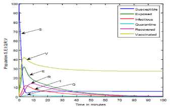
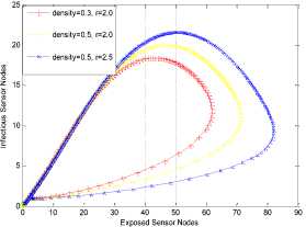
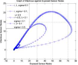
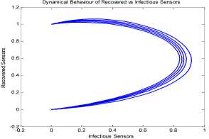
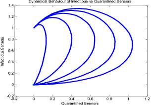
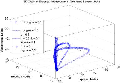
) -
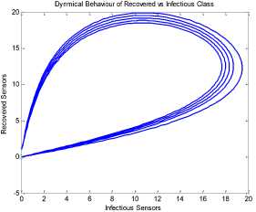
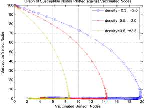
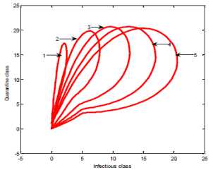
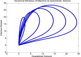
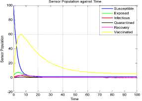
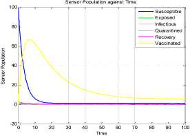
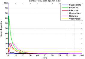
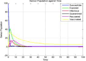
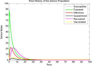
a rf ) (A - S*t - V-*t)(t+)X++t+d ) , , , . , (0+t)(t+ t+ co). (- ail Ф+(- П - t - d )(vp----^9 a(t+ф) , , , . , <0+t)(-t- +v+т+co). (- ail p+(-1-t - d )(v ф - ^---^---^^) R * V*t+S*t - A , (-S-t)(-t - t - d ) (A - S*t - V-0t) m +г , r xr <6+T)<T+^)<a+v + T+CO). Ф (- a rf ф+( -1 - t - d )(v ф - ----—^-) „* _ p(S+T)(a+v+t+d) 1 P S (f+t)<™ ri- Endemic equilibrium Ef = (S*, E* ,I*, Q0, R0, Vf) for Model 2 i.e. Fig.2. Schematic Diagram for the Flow of Worms in WSN E * - S * L2 (S+т)(а+v+t+d ) /?0anr§ (1+t+d )(a+v+t+d )(- t - cp )S*t(^+p+t )/ <0 +т)<т+ co).. < S<-al ф+(- 1 - t - d)(v --0---------)) (t+cp)(1+t+d)( a+v+t+d )S*t(^+p+t)/( f+t)) , , , , ., , , ,, <0+т)<т+ )Va+v+т+ o).. (a+v+t+d )( - a1 cp+( - rj - t - d )(v cp- ---——-^---------)) Q 0 = ( t+p )<1+t+d )(a+v+t+d)(A - S*T . < 0+т)<т+ (1+t+d )(a+v+t+d )( - ap cp+( - rj - t - d )(v p- ---——-^-)) * _ (S+t)(t+p)<1+t+d)(a+v+t+d) R1 л г <0+т)<т+ S p (- a1 p+(-1 - t - d )(vp -1---——-)) A-S *T(f+p+T)/(f+T) Here, we present the analysis for Model 2 (SEIQR-V); note that, стяг02 is replaced with стяг02/L2. The following system of differential equations represents the model; S = Л - PSI акт//L2 - tS - pS + pR + fV E = PSIcmr2/L2- (t + 0)E I = вE - (t + ti + v + «)I (2) Q = «I - (t + ti + p)Q R = pQ + vI - (t + p)R V = pS - (t + f)V B. Solutions of Equilibrium Points Equating the modified system of differential equations to zero we obtain two solutions which are the worm-free V* Ф L2 p (S+t) (a+v+t+d) p6 (f+t) алг2 A cursory look at the symbolic solutions of the endemic equilibrium in Mishra and Tyagi’s analysis shows the differences. It is observed here that the expression for uniform distribution deployment formed part of the solutions; this is absent in their solutions. C. The Basic Reproduction Ratio We apply the method used in Mishra and Pandey [25], therein authors regarded the Reproduction ratio/number as the inverse of the susceptible nodes (S*) at the endemic equilibrium. This method gives the same result with the next generation matrix method for finding the reproduction number (and used in [20]).The Reproduction number for Model 1 and Model 2 are given as follows: ratios involved the parameters of uniform random distribution of sensors and transmission range. This is absent in [20]. D. Stability of the Worm-free Equilibrium Point R= (в+т)(aw+т+а)) R P О СПТГд 0 L2 (0+r)((z+v+t+co) Here, we compare our reproduction ratios for the different topological expressions and the reproduction ratio in derived in [20]. Specifically, our reproduction We show the proof of local asymptotic stability at the Worm-free Equilibrium using the jacobian method. This is done by showing that “the eigen-values of the jacobian matrix all have real parts” [17] or that the “characteristic equation of the jacobian matrix” derived from the system of equations has negative roots [26]. The jacobian matrix of Model 1 is (6), while the jacobian matrix of Model 2 is (7). ⎡–(т+P) 0 -рантах(^+T) T(f+T) 0 0 1 ⎤ 0 –(T+e) Paur^X(^+т) т(f+r) 0 0 0 ⎥⎥ J ( EF0 ) = 0 9 –(T+w+V+a) 0 0 0 ⎥ (6) 0 0 a –(T+w+Л) 0 0 ⎥ 0 0 V n –(T+ ) 0 ⎥⎥ ⎣ P 0 0 0 0 –(T+ ^)⎦ ⎡–(T+p) 0 -POKY^X(^T) L2t(f+T) 0 0 - ⎤ 0 –(T+0) p алг02X(f + T) L2t(^+t) 0 0 0 ⎥⎥ J (EF0 ) = 0 9 –(T+ И/ +V+a) 0 0 0 ⎥ (7) 0 0 a –(T+w+p) 0 0 ⎥ 0 0 V 9 –(T+Ф) 0 ⎥⎥ ⎣ 0 0 0 0 –(T+e)⎦ The eigen values of (6) and (7) are –(T+p),–(T+9), –(T+W+V+a) , –(т+w+Л) , –(T+Ф ) and –(T+{); which all are negative hence the systems are locally asymptotically stable at worm free equilibrium point. IV. Simulation Experiments and Discussion for Model 1 The simulation experiments for the SEIQR-V model were done using these following initial values for the Wireless Sensor network S=100; E=3; I=1; Q=0; R=0; V=0. Other values used for the simulation include Л=0.1; p = 0.1; T=0.003; 0)=0.2; 9=0.3; a = 0.1; p = 0.4; = 0.06; v=0.4; p=0.3; Ф=0.3; adapted from the time history of [20]. Fig. 3 and Fig. 4 [20] are similar in terms of the values of several compartments. However, at Fig. 3 the value for r is 1; therefore our simulation and that of [20] gives similar dynamical behavior at this value. But placing r at 2 (in Fig. 5) showed remarkable difference. Fig.3. Time History at r=1 and о = 0.3 Fig.4. Time History of [20] Fig.5. Time History at r=2 and о = 0.3 : to Time ----Susceptible Exposed Infectious ------Quarantined Fig.6. Time History at r=2 and О = 0.5 The increase in range and density can be seen to increase most especially the exposed and the infectious sensor nodes. This is clearly seen in Fig. 7; where keeping r constant (2.0) and increasing density from 0.3 to 0.5 correspondingly increased the exposed node from above 60 sensor nodes to above 70 sensor nodes and increased the infectious nodes from 17 to 20 nodes. On the other hand, keeping the density constant and (0.5) and increasing r from 2.0 to 2.5 showed corresponding increase for the both the exposed and the infectious sensor nodes. reduced the impact of a countermeasure such as vaccination. Keeping the density constant (at 0.5) and increasing r (from 2.0 to 2.5); then keeping r constant (at 2.0) and increasing density (from 0.3 to 0.5) persistently had a negative impact in the wireless sensor network environment. The real world implication is that as any of these parameters are increased there is a high possibility that the impact of the sensor node inoculation is weakened; and this may cause exposure of nodes to more infection. Observing Fig. 9 [20], one can clearly see that arrow 1 which represents the value of the vaccinated nodes with their time history was reduced to 20 nodes in Fig. 8 as a result of these parameters. Fig.9. Susceptible vs Vaccinated Sensors [20] Fig.10. Recovered vs Infectious Sensors [20] Graph of Infectious Nodes Plotted against Exposed Nodes Fig.7. Infectious vs Exposed Sensors Fig.11. Recovered vs Infectious Sensors Fig.8. Susceptible vs Vaccinated Sensors Fig.12. Infectious vs Quarantined Sensors [20] Fig. 8 shows how the increase in density and the range Fig.13. Infectious vs Quarantined Sensors Fig.14. Simulation result at r, L, о=0.1 Table 2. Values for Plotting Recovered vs Infectious Class Rate of recovery (V) Rate at which recovered nodes become susceptible (ср ) 0.4 0.3 0.42 0.33 0.44 0.35 0.46 0.37 0.48 0.39 Fig.15. Simulation result at r, о=0.1; L=0.5 Table 3. Values for Plotting Recovered vs Infectious Class Rate at which exposed become infectious (9) Rate at which infectious get quarantined (а) 0.3 0.1 0.5 0.3 0.7 0.5 0.9 0.7 1.1 0.9 Comparing Fig. 10 [20] and Fig. 11 shows the impact of our modification; while in the former the simulation result didn’t go past 15 nodes for both recovered and infectious nodes, the latter was almost 20 nodes. On the other hand while Fig. 12 [20] did not go past 20 nodes, Fig. 13 was almost 30 nodes. Note that Fig. 11 and Fig. 13 were gotten using the values of Table 2 and Table 3. Fig.16. Simulation result at r=0.1; а, L=0.5 V. Simulation Experiments and Discussion for Model 2 Here, we would simulate to elicit the impact the effect of transmission range, density, length of side and quarantined in a topology different from Model 1 of SEIQRV. Simulation experiments performed with this model was possible with values listed above, with the exception of L. It is evident from time histories of Model 2 i.e. (Fig. 14, Fig. 15, Fig. 16 and Fig 17) that they are grossly different from Fig 4 of Mishra and Tyagi [20]. This is due to the factors added in the models herein. These time histories also show how sensitive this topological expression is. Fig.17. Simulation result at r,СУ=0.5; L=0.1 Fig.18. Infectious vs Exposed Nodes Fig. 18 shows the dynamical behavior of infectious and exposed nodes. This figure depicts the impact of transmission range, distribution density i.e. the increase the exposed and infectious class. To further show the sensitivity of our addition in this model and its significant difference with the results of [20], we use the values of Table 2 and Table 3. Fig.19. Recovered vs Infectious Sensors Fig.20. Infectious vs Quarantined Sensors The dynamical behaviors of the model shown in Fig. 19 and Fig. 20 are for recovered against infectious sensors and infectious against quarantined sensors respectively. Comparing them with Fig. 11 and Fig. 13 of Model 1 as well as Fig. 10 and Fig. 12 of [20], shows obvious differences that further depict the sensitive nature of the expression applied to the SEIQR-V. Fig. 21 presents a three dimensional phase plane of exposed, exposed and vaccinated nodes using several values; the parameters for transmission range, distribution density and length of side are varied. Fig 22 depicts the time history of model 2 at transmission range of 2, length of side and density of 0.5. This figure is necessary for describing further the numeric implications of reproductive numbers. Fig.21. 3D Phase Plane of E, I and V Sensor Nodes Fig.22. Time History at r=2 and L, о=0.5 At this juncture we generate numeric values of the basic reproduction ratio (Ro) of Section III, subsection C; using Fig. 3, Fig 4, Fig 6, Fig 15, Fig 16 and Fig 22, and the results are presented in Table 4. In generating the actual values of the reproduction ratios, we further demonstrate the impact of our modifications to the original SEIQR-V model (in Mishra and Tyagi [20]) for wireless sensor network. Recall that in epidemiology when the “reproduction number is less than one, the infected fraction of the sensor nodes disappears and if the reproduction number is greater than one, the infected fraction persists” [17]. From the table, it is evident that the reproduction numbers of Fig. 4 [20] and Fig. 3 are almost the same. This shows that at transmission range (of 1) and density (of 0.3) the dynamical behavior of Model 1 herein is similar to that of the model in Mishra and Tyagi [20]. But increasing the transmission range (to 2) and the density (to 0.5), also increased the reproduction number from 0.133 to 0.885. More so increasing the range and density further would verily make the Ro to go beyond 1; which entails an epidemic in the sensor network. Table 4. Time Histories and their Reproduction Numbers Figures Parameters Considered Reproduction numbers Fig. 4 [20] --- 0.140 Fig. 3 Range and Density (Model 1) 0.133 Fig. 6 Range and Density (Model 1) 0.885 Fig. 15 Range and Density (Model 2) 0.002 Fig. 16 Range and Density (Model 2) 0.221 Fig. 22 Range and Density (Model 2) 3.540 The reproduction number of Fig. 15 is less than that of Fig 4 and Fig 3; and it also depicts the impact of range and density (which was reduced to 0.1) i.e. causing the total elimination of worm infection in the sensor network. Note that the expression used for Model 2 involved length of side (L); and this parameter further changed the dynamical behavior of the SEIQR-V epidemic model. Increasing distribution density from 0.3 to 0.5 in Fig 16 gave a Ro of 0.221 and increasing the range from 0.5 to 2 gave a Ro of 3.540. Keeping the range at 2 and reducing the density to 0.3 would give a Ro of 2.12. In order to curb incidences of sensor network epidemic, network security experts ensure that the reproduction numbers is less than 1 at all times. Spurred by the deficiencies of the SEIQR-V epidemic model by Mishra & Tyagi [20], we propose modifications that will allow the inclusion of distribution density and transmission range. This is to present a truer picture of the model and to generate better reproduction numbers for introducing a single infective sensor in a susceptible sensor population. The actual expression used for modifying the SEIQR-V model were culled from these works; [13,14,18,22]. Simulation experiments were performed to elicit the impact of our modifications. Firstly, we noticed an increase in the exposed and the infectious class when transmission range and density was increased. Secondly, we elicited other differences between our results and the results of [20]. Furthermore, we would investigate the impact of vertical transmission, media access control (MAC) and collisions using the SEIQR-V epidemic model. Acknowledgment We thank the anonymous reviewers that read our manuscript and their keen efforts directed at ensuring accuracy of our work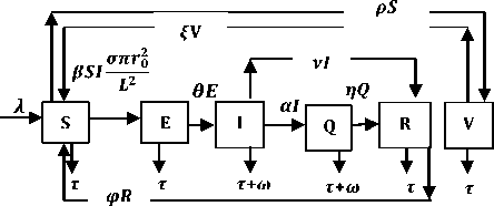

VI. Analyses Using the Basic Reproduction Number (RO)
VII. Conclusion
References The SEIQR–V model: on a more accurate analytical characterization of malicious threat defense
- A. Bröring, J. Echterhoff and Simon Jirka, "New Generation Sensor Web Enablement," Sensors, vol. 11, pp. 2652–2699, 2011.
- S. Yinbiao, K. Lee, P. Lanctot, and F. Jianbin. Internet of Things : Wireless Sensor Networks, 2014.
- C. H. Nwokoye, I. Umeh, M. Nwanze, and B. F. Alao. 2015. Analyzing Time Delay and Sensor Distribution in Sensor Networks. IEEE African Journal of Computing & ICT, vol. 8, pp. 159–164, 2015.
- S. Singh and A. Malik, "Heterogenous energy efficient protocol for enhncing the lifetime in WSNs", International Journal of Information Technology and Computer Science, vol 9, pp. 62-72, 2016
- W. O. Kermack and A. G. McKendrick, "A Contribution to the Mathematical Theory of Epidemics," Proceedings of the Royal Society A: Mathematical, Physical and Engineering Sciences, vol. 115, pp. 700–721, 1927.
- W. O. Kermack and A. G. McKendrick, "Contributions to the mathematical theory of epidemics. ii. the problem of endemicity," Proceedings of the Royal Society of London. Series A., vo1. 38i834, pp. 55–83, 1932.
- W. O. Kermack and A. G. McKendrick, "Contributions to the mathematical theory of epidemics. III. Further studies of the problem of endemicity," Proceedings of the Royal Society of London. Series A, Containing Papers of a Mathematical and Physical Character, vol. 141, pp. 94–122, 1933.
- S. A. Khayam and H. Radha, "A topologically-aware worm propagation model for wireless sensor networks", 25th IEEE International Conference on Distributed Computing Systems Workshops, IEEE, pp. 210–216, 2005.
- S. A. Khayam and H. Radha, "Using Signal Processing Techniques to Model Worm Propagation over Wireless Sensor Networks," IEEE Signal Processing Magazine, pp. 164–169, 2006.
- P. De, Y. Liu, and S. K. Das, "Modeling node compromise spread in wireless sensor networks using epidemic theory," International Symposium on on World of Wireless, Mobile and Multimedia Networks, IEEE Computer Society, pp. 237–243, 2006.
- P. De, Y. Liu, and S. K. Das, "An epidemic theoretic framework for evaluating broadcast protocols in wireless sensor networks. 2007 IEEE International Conference on Mobile Adhoc and Sensor Systems, IEEE, pp 1–9, 2007.
- P. De, Y. Liu, and S. K. Das. 2009. Deployment-aware modeling of node compromise spread in wireless sensor networks using epidemic theory. ACM Transactions on Sensor Networks (TOSN) vol. 5, pp. 3-23, 2009.
- S. Tang and B. L. Mark, "Analysis of virus spread in wireless sensor networks: An epidemic model," Proceedings of the 2009 7th International Workshop on the Design of Reliable Communication Networks, DRCN 2009: pp. 86–91, 2009. http://doi.org/10.1109/DRCN.2009.5340022
- X. Wang and Y. Li, "An improved SIR model for analyzing the dynamics of worm propagation in wireless sensor networks," Chinese Journal of Electronics, vol. 18, 2009.
- X. Wang, Q. Li, and Y. Li, "EiSIRS: A formal model to analyze the dynamics of worm propagation in wireless sensor networks," Journal of Combinatorial Optimization, vol. 20, pp. 47–62, 2010. http://doi.org/10.1007/s10878-008-9190-9
- S. Tang, "A modified SI epidemic model for combating virus spread in wireless sensor networks." International Journal of Wireless Information Networks, vol. 18, pp. 319–326, 2011.
- B. K. Mishra and N. Keshri, "Mathematical model on the transmission of worms in wireless sensor network," Applied Mathematical Modelling vol. 37, pp. 4103–4111, 2013. http://doi.org/10.1016/j.apm.2012.09.025
- Y. Wang and X. Yang, "Virus spreading in wireless sensor networks with a medium access control mechanism," Chinese Physics B, vol. 22, 40200-40206, 2013. http://doi.org/10.1088/1674-1056/22/4/040206
- B. K. Mishra, S. K. Srivastava, and B. K. Mishra, "A quarantine model on the spreading behavior of worms in wireless sensor network. Transaction on IoT and Cloud Computing, vol. 2, pp. 1–12, 2014.
- B. K. Mishra and I. Tyagi, "Defending against malicious threats in wireless sensor network: A mathematical model", International Journal of Information Technology and Computer Science, vol. 6, pp. 12–19, 2014.
- Z. Zhang and F. Si, "Dynamics of a delayed SEIRS-V model on the transmission of worms in a wireless sensor network," Advances in Difference Equations: 1–15, 2014. http://doi.org/http://www.advancesindifferenceequations.com/content/2014/1/295
- L. Feng, L. Song, Q. Zhao, and H. Wang, “Modeling and stability analysis of worm propagation in wireless sensor network. Mathematical Problems in Engineering 2015.
- C. H. Nwokoye, V. E. Ejiofor and C. G. Ozoegwu, "Pre-Quarantine approach for defense against propagation of malicious objects in networks," International Journal of Computer Network and Information Security (IJCNIS), vol. 9, pp. 43-52, 2017. doi:10.5815/ijcnis.2017.02.06
- C. H. Nwokoye, V. E. Ejiofor, R. Orji, I. Umeh, and N. N. Mbeledogu. Investigating the effect of uniform random distribution of nodes in wireless sensor networks using an epidemic worm model. CORI'16, pp. 58-63, 2016.
- B. K. Mishra and S. K. Pandey, "Dynamic model of worms with vertical transmission in computer network," Applied Mathematics and Computation, vol. 217, pp. 8438–8446, 2011.
- B. K. Mishra and A. Singh, "Global Stability of Worms in Computer Network," Applications and Applied Mathematics,An International Journal vol. 5, pp. 1511–1528, 2010.
