The Study of Joint Acoustic Holography Algorithms based on Continuous Scanning

For military torpedoes, ships and other large underwater vehicle, it is very time-consuming for the acoustic holography measurement. To effectively solve this problem, this paper proposes a continuous scanning method for rapid measurement. This makes the measured radiated noise with Doppler effects. And then the traditional method of sound source identification is difficult to efficiently identify the noise source localization. Because the near-field acoustic holography can be used not only to reconstruct Volume of three-dimensional sound field with two-dimensional information and can also improve the spatial resolution and the accuracy of volume of the sound field reconstruction with the use of the missed wave information. So scholars from home and abroad launch a research on the acoustic holography method in the application of sound source identification.

Abroad, Kim and Park use mobile framework technology to analyze vehicles of the sound field and apply the vehicle acceleration of the sound field [1]-[5]. At the same time, the problem that phase error compare with the amplitude error is more prone to distortion radiated sound field can be solved through the correction factor to reduce the speed of sound source movement phase error. R.J.Ruhala and David C.Swanson conducted a research of the plane acoustic holography technique in a moving medium and application to moving medium form of Green's function is proposed [6]. In China, Yang Diange and Luo Yugong proposed the theory based on the near-field acoustic holography method of moving acoustic source identification [7] [8]. The research which uses Elimination of time-domain Doppler principle and near field acoustic holography principle to reconstruct moving sound field can realize the exact identification of moving sound source. On the whole, the use of acoustic holography method of moving noise sources are adopted to eliminate the Doppler effect on the signal processing and use the reconstruction formula for proper reconstruction of acoustic noise sources of information.

Considering of the mobile framework technology can quickly get space of discrete sampling points and the HELS method is applicable to the reconstruction of the sound source of arbitrary shape[9]-[12]. It has the characteristics of a simple realization, computation and the reconstruction results of high precision. In this paper, a combination algorithm is applied to any shape moving source of sound field reconstruction. This method first obtain the amplitude and phase correction of the space of discrete sound pressure values with the mobile frame technical analysis and then use HELS reconstruction methods on the field to finish the exercise of arbitrary shape identification and location of sound source.

HBasic principles

A HELS Algorithm

With density ρ ₀ , sound velocity c in the infinite fluid medium, considering any structure of the acoustic radiation and using HELS method, we can write any point of sound pressure p ( x , ω ) [9]:

p (r, to) = £ Cj tj (r, to) (1) j=1

V j is a pressure basis function under the coordinates. For example V j can be written in the spherical coordinate system:

^T j = V n , l ^{( Г} , ⁰, Ф) = h n ^{( kr} ) ^Pn , l (cos ⁰e^ (2) Which k = to / C is wave number, h n is Spherical Hankel function, P_{n , l} is Associated Legendre function, the relation among the values of j , n , l : j = n ² + n + l +1 , l changes from — n to n .

The coefficients C_j that assumption ( 1 ) match with rr

X m of the sound pressure p ( X m , to ) measurement points, which is m = 1,2, K , M ( M >  J ) , are written in matrix form:

{P(Xm ,to)}M x1 = [T]MX J {C} JX1       (3)

If the matrix is ill-condition, (3) can be solved by singular value decomposition, otherwise, it can use the method of generalized inverse coefficient to obtain C _j : r

^{{ С }} J x 1 = ^{([ T} ] M X J ^{[ T ]} MXJ ) ^{[ T ]} MXJ ^{{ p ( X}m , ® )} M x 1 /дч

= W { p ( X „ , to )} M x 1

Where W = ([^] M x J [T M x J Г^ ] M x J , once make sure the coefficient C _j , (1) can be used to sound pressure reconstruction.

B Doppler effect

But when the noise source is moving acoustic source and according to the theory of Morse Moving Sound Source, If the sound is emitted by point source:

q (t) = qо e11"—kr)/ r sound pressure signal pi (t) which measured by the i hydrophone in the receiver array can be expressed as:

₍ t ) = 1    q [ t — ( RJ c )] + q (cos 0 — M)V

^P1     4n R i (1 — M cos 0 )² 4 n R , ²(1 — M cos 0 i )²

The first part of equation (5) is acoustic radiation item in accordance with the propagation distance decay, and the second part is proximity effect. When velocity of the sound source is low and Mach number is lower than 0.2, the second part is much smaller than the first part. And then can be ignored, the received sound pressure can be reduced to:

p (t) =      q[t—(R/c)]4n Ri (1 — M cos0)2

which

R =

Mxi + xx+ + (1 — M 2)(У2 + zl)

1 — M 2

cos 0 i

x_i R i

Which [ x_i , y_i , z_d ] is the coordinates of the i sensor, M is Mach number. Then the expression of acoustic particle velocity can be obtained:

u,( t) = Pi( t)/ZOi (7)

Where Z _{0 i} is spherical wave impedance which is responding to the i sensor.

Contrast to the sound pressure expression of point source, it can be seen that movement makes the error exists between amplitude and phase of signal which is received by sound pressure hydrophone. Take the pressure signal as an example: in the measurement it can be assumed that the actual measured complex acoustic pressure pˆh is equal to complex sound pressure of stationary source p and noise term pe caused by motion. It is shown that:

Ph = P + Pe

（ 8 ）

Take equation ( 8 ) into ( 4 ) , then the coefficient of each basis function { C } J _{x 1} can be expressed by :

{C} J X1 = Wp + WPe           (9)

W = ([^] M X J [^] M X J ) ^— 1 [^ ] M X J . Using this factor to reconstruct the sound field will obviously bring error. In the reconstruction of sound field, sound pressure can be expressed as:

ps = ^'c = ^ 'Wp + ^ 'Wpe        (10)

^ is the basic function matrix of reconstruction surface. p s =^ Wp is the pressure in reconstruction sound;

Errors : (ps)e = ^ Wpe , then relative error of reconstruction pressure can be shown as:

（ 11 ）

Using the fundamental theorem on the norm-type the above equation can be simplified as:

< cond (T W )

p e

（ 12 ）

Condition number cond (T W ) is relative with the selected measurement coordinates, the coordinates of reconstruction surface and the number of basis functions. When the sound source movements generate the sound pressure amplitude and phase error, it certainly brings the error to reconstruction sound pressure. And from equation (12), it is shown that the greater the velocity the greater error of measurement data and the reconstruction pressure.

C Mobile Framework Technology

The method follows the introduction of the three coordinates, see Fig.1 [1] [2].

Which   Phol   is the wave number of frequency fh .Equation (16)、 (17) can deduce：

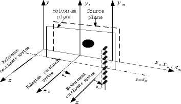
Fig.1 the measurement of coordinates

1 " ^  2n(f — f)

FT {Phol ("m/ ht • Ук • ZH; t)}=    j Plol(           • Ук • ZH; fh )dfh

—”

m / h               m / h

Suppose the figure ( x , y , z ) is the reference coordinate system, ( x_m , y_m , z_m ) is hydrophone array in the measurement coordinate system, ( x_h , y_h , z_h ) is hologram plane coordinate system with the goal of movement. For any moment t , the following relationships between the various values in the three coordinates are:

The above equation is the basic theoretical formula of mobile framework technology. The left part of (18) is the Fourier transform of measurement signal in time domain, and the integrand on the right is wave-number spectrum of the Doppler shift in the x direction

However, this method only applies to single-frequency sound source. When the sound field is given by a single frequency point source, equation (18) can be simplified:

Ft{p„ ("„t• Ук • zH; t)}/4/h =—Po (2^^ • Ук • zH; fh)

Un m / h            m / h

The anti-type Fourier transforms time-domain of the above equation

( y= =    ， z= =    ， x= =          ) (13)

y m y h      m h m m h h

Definition of measurement coordinate system and the relative speed of holographic coordinates are "_m / h = "_m — " h • sound pressures in the three coordinates are:

Pmc (xm• Уm• ZH ; t) = Phol (xh• Ук• ZH; t) = Phol(xm + "m/ ht• Ук• ZH; t)

Which p_mic ( x_m , y_m , z_H ; t ) is sound pressure of hydrophone measurement; p_M ( X m + U m / h t , У m , Z h ; t ) is sound pressure of holographic plane. Generally order X m = 0 , at this point hydrophone fixed and the target move, (13) can be simplified to:

¹ ˆ ^Phol

u m / h

(w, —f)

V " m / h

X

ˆ

• У к • Z h ; f h =    F T4 P ho

u m / h

(20) is submitted to (19)

2^f

\1

25- • У к • Z h ; f h e —j*

V " m / h

7J

=£ P ho (k x • У к • Z h ; f- ^ e' x x h dk 'e —^ = P ho (. ^xh • ^Ук • ^zh ^; f h ) e j 'n' h

Pmic (0, Ут • ZH ; *) = Phol (um/ht• Ук • ZH ; *) (15)

It is shown the relationship between measuring signal and holographic coordinate. The left side of the equation is the hydrophone received time-varying sound pressure signals which have Doppler shift. The right side of the equation is the holographic coordinate which is corresponding to the measured signals in time. The time-domain Fourier transform of the holographic surface acoustic pressure:

P hoi ( x h • У к • ^z h ; fh ) = P mc (o> У к • ^z h ; t ) e^{j 2 n}f h * / ^{A f}

This is an important derived equation for mobile framework technology. This equation shows that: when the frequency of sound source is known, the value of the spatial distribution of sound pressure on holographic face can be abstained by multiplying e j ^ f h * with hydrophone received signal in time domain. Space time-domain signal can be translated into a signal of planar point by mobile framework technology, Meeting the data requirements of HELS method, the processed data can be use as the input data of HELS method, which can constitute a combination of moving sound source based on HELS algorithm.

FT {phol(um/ht, yh, zH;t)}

=Г I" Phol("m/ht• Ук• zH; P)e—j2'fh'dfe*2''fd (16) —" —"

Which P_hol is the spatial distribution of sound pressure at frequency f_h . The sound pressure wave number spectrum is Fourier transform of its airspace:

Phol(Xh = "m/ht• yк • ZH; fh )

"

1      Phol(kx,yh,zH;fh)ejkxxhdkx

2 n ^— "

Ш The investigation of Simulation

Selecting the most representative of the point source to be simulated, simulation model is shown in Fig.1. A point sound source does uniform motion at 1m / s speed along the x-axis. And the motion time is 1.6s.The scan range of x-axis direction is ( 0-1.6m ) .The minimum distance between linear measurement array and sound source and measure is defined as the measuring distance: zm=0.1m( X / 6 ). The Doppler effect of time-domain

signal is acquired by a 12 fixed uniform linear array. The distance between hydrophones is 0.075m ( X /8 ). The coordinates of linear geometric center is ( x=0.8,y=0,z=0.1 ) . The scan range of y-axis direction is ( -0.4125m-0.4125m ) . The location of sound source is ( x=0.8,y=0,z=0.1 ) . when there are two sound sources, their locations are ( x=0.6,y=-0.2,z=0 ) and ( x=1,y=0.2,z=0 ) . To compare with the accuracy of sound field reconstruction ， assuming the stationary sound source and the linear array geometric center are located in the z-axis ， the theoretical value of the sound field is calculated at the horizontal distance in the plane zh = 0.05m.

For visual representation to the accuracy of sound field reconstruction, p _s is the theoretical value of measuring sound pressure and p _r is the calculated value of sound pressure reconstruction. Define the relative percentage of the sound pressure amplitude error as: norm ( p, - p )

L = 100 X sqrt (        r—^ )      (22)

norm ( p_s )

• TABLE 1

RECONSTRUCTION ERROR OF SOUND PRESSURE AS

DIFFERENT FREQUENCY FROM SINGLE SOURCE

F(kHz)     2.5    3.15     4       5      6.3      8      10

L error (%)     0.18    0.14    0.22    0.22    0.52    0.89    0.16

Table1 shows that the combination algorithm is particular for spherical sound source. And a wide frequency range of the sound source can be analyzed. Because HELS is based on the principle of the spherical wave superposition and sound field approximation. The single point source and spherical sound source can be a very high similarity which can get high accuracy sound field reconstruction.

• TABLE 2

RECONSTRUCTION ERROR OF SOUND PRESSURE AS

DIFFERENT FREQUENCY FROM DOUBLE SOURCES

F(kH     0.1      0.5       1       1.6       2       2.5     3.15

z)

L error (     7.9     7.96     7.82     9.4     11.2     16.6     40.7

%)

Table2 shows that when there are multiple noise sources in the complex sound field, the combination algorithm has some limitations with the sound source frequency. It can only more accurately reconstruct the sound source frequency which is less than equal to 2.5 kHz. But it can ensure the accurate identification of noise source positioning, so the combination algorithm can analyze radiated acoustic field of any shape motion noise sources.

IV The investigation of experiment

A Experimental measurement of moving acoustic source holography

To verify whether the established combination acoustic holography of continuous scanning is effective, two standard transmitter transducer sound sources are selected as the research object. This method is applies to reconstruct the sound field, and the actual results were compared in control.

The test is conducted in an anechoic basic, and the measuring model parameters are the same with the study of simulation. Pressure array is installed in the mechanical support of automatic scanning system by the boom. It is scanned by the mechanical support which is controlled by the computer software or manual. Its location accuracy is 2mm. The sound sources are spherical transducers, and its radiuses are Г 1 = 0.04 m , Г 2 = 0.06 m . The selected transmission frequencies are 3.15kHz 、 4kHz 、 5kHz 、 6.3kHz. 12 pressure hydrophones are fixed in a glass steel array. The length of array is 0.825m, the distance between the array elements is 0.075m which is shown in fig2. The array is vertically distributed on the pool. The distance from the top of array to wedges on the surface of pool is 0.9m. And the distance from the bottom of array to wedges on

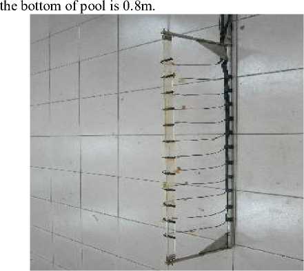
Figure 2 the array of press

The diagram of sound source and sound pressure array basic can be seen in Figure 3, Figure 4. Fig3 is the experimental condition of the single sound source. The spherical emission transducer is fixed in a dipping rod. With its geometric center as the origin of reference coordinate system, the distance between the sound source and the surface of water is 1.8cm. the distance from the sound source to the horizontal array (z axis) is: zm = 0.05m(0.1 m, 0.15m). The movement range of array in x direction is -0.8m : 0.8m . First, the mechanical frame is marked on the ruler. Then after several measurements the aircraft movements can be obtained at2.67cm/s . Because the speed error has a great influence on the sound field reconstruction, the aircraft movements for the uniform motion is tried to ensure.

Fig4 shows the experimental condition of two sound sources. According to the settled coordinate system, the distribution of two sound sources are ( -0.2 ， 0.2 ， 0 ) and ( 0.2 ， -0.2 ， 0 ) . The big ball is 1.6m from the surface of water and the small ball is 2.0m from the surface of the water.

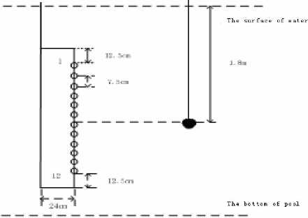
Fig.3 sketch map of holography measurement

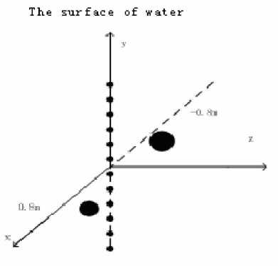
Fig.4 sketch map of double sources arrangement

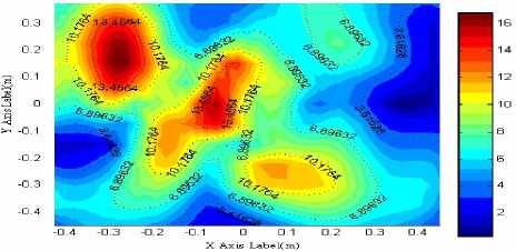
(b)the reconstruction pressure(pa)

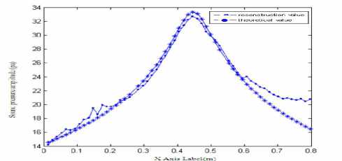
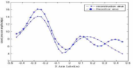
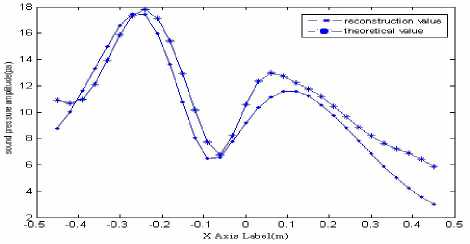
(c) x-axis profile

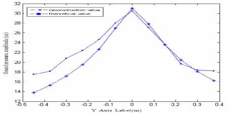
(d) y-axis profile

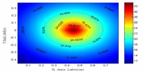
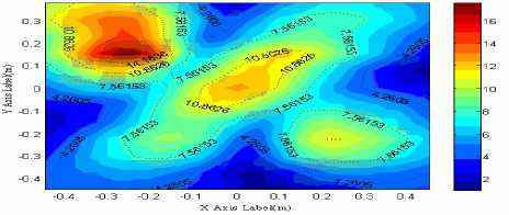
Fig.5 Theoretical and reconstruction value of sound pressure at frequency f=2.5 kHz

• TABLE 3

RECONSTRUCTION ERROR OF SOUND PRESSURE AS

DIFFERENT FREQUENCY

F(kHz) 2.5    3.15         4         5   6.3

L error (%)   8.80   7.18   4.89       5.30       4.66

B Analysis of test data and results

Those are the reconstruction results of single sound source

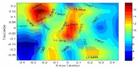
(a) the theory pressure(pa)

Fig5 (a) shows sound field distribution of single sound source when the frequency is at 2.5 kHz. Fig5 (b) shows reconstruction distribution of sound pressure in the sound field. So the combination algorithm can accurately identify and locate the noise source. See from table3, sound pressure amplitude relative error of sound field reconstruction is below 10%, and reconstruction error is not linear with frequency, but at some point there is the minimum, which is corresponding with the characteristics of least squares. Because the transmitter transducer selected in the experiment is spherical, this meets with the scope of Helmholtz equation least squares (HELS). And superposition of spherical wave can be better approximation of the sound field. Therefore this method is particularly suitable for analyzing radiated acoustic field of ball sports noise sources.

Those are the reconstruction results of multiple sound

sources

(a) the theory pressure(pa)

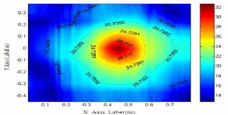
(b)the reconstruction pressure(pa)

are the magnitude errors. The sound pressure amplitude error of sound field reconstruction is 23.9848%. But when the sound source frequency is more than 2500Hz, accuracy of sound field reconstruction is sharply increasing. Distribution of the sound pressure reconstruction can not reflect both the size and location of sound sources. And there is no meaning when the sound field reconstruction error is close to 100%. This result is corresponding to the simulation. Because the array of the two point sources is similar to a long-type sound source. When the ratio of sound source is deviated from ( 1 ： 1 ： 1 ) , the results that using spherical wave expansion of the reconstruction are poor.

Those are the inversion results of different measurement surface

For the moving sound source, there only discusses the length of the array direction on the impact of the moving sound field. When the number of measurement matrix is n=12, 10, 8, accuracy of sound pressure field reconstruction and location analysis are discussed. Supposing the size of the two source surfaces is 0.4 x 0.4, the ratio of the direction of measuring surface measurement array and the source surface under these three cases are: 2.06, 1.69, 1.31, and 0.94.

(c) x-axis profile at y=0.15

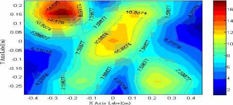
(a) the theory pressure(pa)

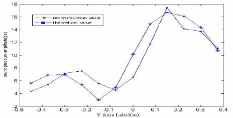
(d) y-axis profile at x=-0.27

Fig.6 Theoretical and reconstruction value of sound pressure at frequency f=2.5 kHz

(b)the reconstruction pressure(pa)

See from Fig6, radiated acoustic field of multiple moving sound sources are more complex than a single sound source. There are both the sound source and the peak superimposed. The simulation shows that combination of acoustic holography has certain requirements about the frequency of the sound source: Under the measurement model and when the ratio of sound source frequency is not more than 2500Hz, sound source location can be accurately identified despite there

(c) x-axis profile at y=0.15

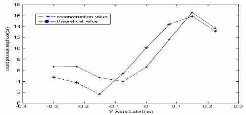
(d) y-axis profile at x=-0.27

Fig.7 Theoretical and reconstruction value of sound pressure as Sm/Sh=1.31

TABLE 4

SOUND PRESSURE AMPLITUDE ERROR UNDER THE

DIFFERENT RATIO OF MEASURING SURFACE AND SOURCE

SURFACE

s m / s h S	2.06	1.69	1.31	0.94
幅值误差	23.9%	23.8%	23.9%	675%

Fig. 7 shows that when the ratio of measuring surface and source surface is 1.31, noise sources can be better identified and located. Seen from Table 4, when the ratio of two surfaces is 2.06, the error of sound field reconstruction amplitude is small, but the plane error is slightly bigger. Because when the sound source frequency is at 2.5 KHz, measurement environment has not met the conditions of infinite space. Reflected waves from bottom and surface have a greater impact on the measurement signals at both ends of the array. Reducing the measurement surface is to remove the array elements at both ends which is equals to reduce the reflection of sound waves on the sound field. Therefore, the accuracy of sound field reconstruction is slightly improved. And when the surface ratio is at 1.69 and 1.31, both the sound field reconstruction results are close and the error is only about 23%. So the method of combining acoustic holography requires low measuring surface size. Using small aperture array which can obtain high precision can provide convenience of engineering applications.

C ONCLUSION

Combination of acoustic holography method based on MFAH and HELS is investigated and verified to measure rapidly the large underwater sound source through the basin test. Noise source identification of location and sound field reconstruction are accurately realized. Workload, time-consuming and other shortcomings which are brought by the traditional way of progressive scanning measurement are effectively solved. Through a series of numerical simulation, the following conclusions are:

• (1)    The combination method only applies to a lower

frequency. When at a higher frequency, the singularity of the transfer matrix is more serious. Numerical solutions are more deviation from the theoretical value and the error is greater.

• (2)    The combination method can reconstruct the radiation sound field of any shaped noise source, and ensure the accuracy of the reconstruction.

• (3)    The combination method has a lower requirement on measuring surface. When the ratio of measuring surface and sound source surface is only 1.3, better reconstruction can be obtained. And the result is similar to the ratio of two surfaces at 2. A small measure surface and quickly identify localization of the noise source are achieved. This advantage is very beneficial to the combination of acoustic holography method in engineering application.