The use of wavelets in the mathematical and computer modelling of manufacture of the complex-shaped shells made of composite materials

It’s well known that composite materials are not only the substances of our future, but also of our present clay. Due to a complex of unique features, including the ability to form these features in the course of production, composites can be used in the various industries. CM have its extensive application in the construction industry, road, housing and utilities sectors, automotive and aviation manufacturing, production and transportation of oil and gas, also for the manufacture of sports equipment and articles of domestic use. To reduce production costs and time for design work and for control parameters of products, enterprises widely apply CAD/CAM/CAE-system.

In the modern CAD/CAM/CAE-systems the geometric modelling of objects and computer solution of geometrical and engineer graphics problems are central. When an object is created, the geometry of the object and its component parts are to be formed in the first place, then the other problems of designing, manufacturing and technology need to be solved. At the same time in the CAD/CAM/CAE-systems special attention is paid to the improvement of the three-dimensional geometric modelling technology. International industry standard for the design of complex curved surfaces is modelling technique based on NURBS. However, the main problem here is not so much the process of modelling itself, as ways to modify and optimize the created geometric patterns that are very critical for the iterative design mode. Therefore, the improvement of the methods of geometric modelling of three-dimensional objects using the CAD/CAE/CAM-systems’ standard mathematical apparatus along with the adapting these methods for specific industrial applications are the actual problems nowadays.

The Russian CAD/CAM/CAE-systems for manufacturing composite structures made of fibrous materials operate with surfaces of revolution and don’t consider the structure of the tape. In such systems, the tape is identified with a thread so its width and thickness aren’t taken into account. The article [4] provides us the mathematical model of the variable width tape winding without regard to its thickness. In this paper, due to the application of semi-orthogonal wavelet systems on a segment some of the geometric modelling algorithms are summarized and the mathematical simulation of laying out the variable width tape with regard to its thickness is constructed. The surface defined by its point frame of sections is considered as the surface of the mandrel.

1. Wavelet System on a Segment Based on the B-Splineof the Arbitrary Order

For geometric applications let us consider the real spaces L2(R) and L2[a; b]. Consider the real functions defined on the segment [a; b]. Suppose that the function ф E L2(R) satisfies the scaling relation [7] ф(x) = V2 ^ ukф(2x — k), uk E R and has a compact ke support. Let фjk(x) = ф(2jx — k). x E [a; b], j,k E Z. It is clear, that for every j there’s only a finite number of such different from zero functions on the segment [a; b]. For definiteness, let these functions be denoted by фj, 0, фj, 1, ...,фj,nj _ 1. Consider [2] the sequence of subspaces Fq С V1 C ... of the space L2[a; b].

Vj    ^lin{фj, о , ^фj, 1 , . . . , ^фj,n j — 1

n j - 1

asφj,s s=0

: as E R , s = 0 , 1 ,... ,n — 1

dim Vj = nj.

n j - 1

So far as Vj- 1 C Vj, then фj_— 1 ,_k = V pjskфj,_s. Introduce the notation [2] Ф j ( x ) =

⁽ фj, o^{( x} ) ф i^{( x} ) ^,...^,фj,n j — 1^{( x} ))• ^p j = ⁽ Pjs,k ) n =o1 k =^ 1 — 1- T!ien ^ф j- 1 = ^ф j ^p j. We denote Wj 1 as the orthogoira .1 complement to Vj 1 iii Vj. Sir ice Vj = Vj- 1 Ф Wj- 1 arid Wj- 1 C Vj. then Wj- 1 is a finite dimerisional space. If Wj = lin{^j, 0 , ^j, 1 ,... ,^j, m j - 1 }, dim Wj = mj. n j - 1

then cj 1 , _k = V qjk фj, _s. Functions ^j, _k are called wave lets and spaces Wj are named s =0

wavelet spaces [6]. Introduce the matrices [2] Ф j ( x ) = ( cj, ₀( x ) , ^j, 1( x ) ,...,^j mj _ 1( x )), Q j = ( q^j,_k ) n-m j - ¹ 1. Tl ien Ф j- 1 = Ф j Q j. It should lie noted, that nj + mj = nj ₊₁.

Let f E L2[a; b] and Пj : L2[a; b] ^ Vj is a, projector. Tlieii the approximation Пj f can be expanded into a rough approximation Пj- 1 f clarifying addend ПW1 f nj-1                                   nj -1 -1                  mj -1 -1

^П j ^f = 52 cj’k^фj’k = ^П j- 1 ^{f + П} W 1 ^f = 52 cj — 1 ’k^фj— 1 ’k ⁺ 52 dj- 1 ’k^j- 1 ,k.

k =0                                  k =0                    k =0

Consider the two vectors of coefficients Cj = (Cj,0,..., Cj,nj—1)T, Dj = (dj,0,..., dj-nj_ 1)T. First one describes the approximation of the function f and the second represents the wavelet coefficients that characterize the deviation Пj- 1 f from Пjf. As shown in [2] Cj = PjCj-1 + QjDj-1. According to this equation the approximation Пj f can Ire restored with a rough approximation Пj- 1 f and wavelet coefficients. Since the linear operators (projectors) Vj ^ Vj- 1. Vj ^ Wj- 1 are defined Irv some matrices Aj, Bj. then Cj- 1 = AjCj. Dj- 1 = BjCj. By wavelet transform of the function f we mean the finding of vectors Cq , D0, D1,..., Dj- 1. It is known [2] the relatiouship between the matrices A j, Bj and p j, Q j

(в j ) = (^P j ^Q j )    .

The matrix Q j in [2] is defined from the homogeneous system of linear equations T j Q j = 0, where T j = P T [(Ф j, Ф j )] and [(Ф j, Ф j )] = (( фj,_i,фj,_s )) ns ₀ is a matrix of scalar products. The matrices Q j a nd P j are known as synthesis filters. The matrices A j a nd B j are known as analysis filters. The set { P j, Q j, A j, B j} is called a filter bank.

In the article [3] the above approach to constructing wavelet systems on the segment is applied to the case when the function ф ( x ) is selected as a B-spline of arbitrary order n. Briefly mention the main results obtained in the paper. We define B-splines of order n as the convolution [6]

1 , if x G [0; 1): 0 , if xG [0;1).

N = Nn— i * N о , N q ( x ) =

Here we note some known properties of B-splines [6]. Firstly, Nn ( x ) >  0 , Vx . Secondly, supp Nn ( x ) = [0; n + 1]. As it is shown in [9], the function Nn ( x ) satisfies the scaling relation

Nn ^{( x} ) = ^ pk^{Nn (2 x} - k ) , ^Pk = Cn ⁺¹ = k i(( + 1 — k )i .

The constructions presented in [3], can be summarized in two following lemmas.

Lemma 1. The function ф ( x ) = Nn ( x ) determines the sequence of subspaces ^Va,-n ^G Va,—n +1 G . . . , ^Va,j ^lin{фj,—n^{, ф}j,—n +1 , • • • , ^фj, 2 ja ( n +1) — 1 ^} ^V ^{L [0; a ( n + 1)]} , a = 1 , 2 ,.... wlьстс u +=0 V_a,j = L²[0; a ( n + 1)].

k +1

Let Xm,k = j Nn(z)Nn(z — m) dz. m = —n,..., n, k = 0, 1,..., n and wi,k = wk,i = k n                           n-k                                                         n

S   Xk-i,s- 6i,k = 6k,i = S Xi-k,s- 1 < i < k < n. Designate qk = q-k = S Xk,s, s=n—i+1                        s=0                                                        s=k k = 0, 1,... ,n p=J( P 0 ,P 1 ,...,Pk ,Pk ,...,p 1 ,p 0, 0,.••, 0) T,        ifn = 2 k p G R2 j a (n+1)+n

.

I ( p о ,p 1 ,... ,pk ,Pk +1 ,Pk,... ,P 1 ,P 0 , 0 ,..., 0) ^T, if n = 2 k + 1.

We define the shift operator Rs : R m ^ R m by the following rule

{ ⁽⁰ , . . . , ⁰ , a 1 , . . . , ^am—s ) ,

( a|s| +1 , ...,am, 0 ,..., 0) T,

if m > s >  0:

a = ( a 1 ,..., am ) .

if —m < s <  0.

If |s| > m. then Rs a = 0.

Lemma 2. The matrices Pj a nd [(Ф j, Ф j)] for the sequence of sub spaces Va, о C Va, 1 C • • • arei

^P j = fn ⁽ R-n p , R-n +2P , • • • , Rn- 2+2 ja ( n +1)p) ,

[(Фj, Фj)] = 2j (di,• • •, dn, q, R1 q,..., R2ja(n+1)-n-iQ, ui,..., un)T, where d S      (^ 1 ,s, ^ 2 ,s, • • • , ^n,s, qn-s +1 , • • • , qn, 0 , • • • , 0) ,  u s      (0 , • • • , 0, qn, • • • , qs, 01 ,s, • • • , 0n,s)

q     (qn, qn-1, • • • , q 1, q0, q 1, • • • , qn-1, qn, 0, • • • , 0) G R

The transpose of a matrix T j = P T [(Ф j, Ф j )] = 2 j ( ti,_s )^ О ^ n ^{+1)+ n, 2 3a ( n +1)+ n} is

TT = 2j (L1, • • • , Ln, w, R2w, . . . , R2ja(n +1)-2n-2w, L2j-1 a(n+1)+1, • • • , L2j-1 a(n+1)+n), where w = (pTR-2nq, pTR-2n+1q, • • •, PTRn+1q, 0,..., 0)T G R23a(n+1)+n,

L i = (( R-n +2 i- 2 p) ^T d1 , ..., ( R-n +2 i- 2 p) ^T d n, 0 , • • • , 0) ^T + ( Rn ◦ R- 3 n +2 i- 2)w , i = 1 ,...,n, L i- 2 3- 1 a ( n +1) + 1 = (0 , • • • , 0 , ( R-n +2 i p) T U1 , • • • , ( R-n +2 i p) T u n ) T + ( R-n ◦ R-n +2 i )w , i = 2 j^{- 1} a ( n + 1) , • • •, n — 1 + 2 j^{- 1} a ( n + 1) .

Using lemma 2, we can find 2 j^{- 1} a ( n + 1) linearly independent solutions h _s = ( h ₁ ,_s,h ₂ ,_s, • • •, h ₂ 3 _a ( _{n +1})_{+ n},_s ) T of the system of linear equations T j h _s = 0. These solutions represent columns of the matrix Q j = (h₁ , •••, h₂ 3- 1 _a ( _{n +1})). We look for the columns h _s so that the functions ^j,_s ( x ) = Ф j ( x )h _s are the shifted versions of the same function, i.e are of one form (except, of course, the boundary wavelets). According to the matrix T j in lemma. 2. this can be done as follows [3]. First consider the case n = 2 k. Introduce the abbreviated notation for matrices composed of elements of the matrix T j-.

Tj

i 1 , j 1 ,.

.,i k .,j m

ti 1 ,j 1      ^{. . .}     ti 1 ,j m

ti k ,j 1     ^{. . .}    ti k ,j m

For internal wavelets (the support is contained in the segment [0; a ( n + 1)]) consider ^h s = ⁽⁰ , • • •, ⁰ , h 2 s-n- 1 ,s, • • •, h 2 s +2 n- 1 ,s, ¹ , ⁰ , • • •, ^{0) T}, s = n + ¹ , • • •, ^{2 j 1 a (} n + ^{1) —} n, where Tj (_{2 s}---^, ₁ ', 3 ^s + n +2 _s ) ( h 2 s-n- 1 ,s, • • •, h 2 s +2 n- 1 ,s, 1) ^T = 0. The remaining 2 n of solutions corresponding to the boundary wavelets choose as follows. For i = 1 , 2 ,...,n < OHSidei ^h n-i +1     ⁽⁰ , • • • , ⁰ , ^hn-i +1 ,n-i +1 , • • • , ^h 4 n +2 - 2 i,n-i +1 , ⁰ , • • • , ⁰⁾ • ^h2 ³- ¹ a ( n +1) -n + i

⁽⁰ , • • • , ⁰ , h 2 ³ a ( n +1) - 3 n- 1 - 2 i, 2 ^{3- 1} a ( n +1) -n + i, • • • , ^h 2 ³ a ( n +1)+ i, 2 ^{3- 1} a ( n +1) -n + i, ⁰ , • • • , ⁰⁾ T, where

¹ ,..., ³ n + ^{1 -}i                                              ^T

Tj n+1 -i,...,4n+2-2i) (hn-i+1 ,s, • • • , h4n+2-2i,s)  =0, s = n i + 1, s-n,...,s+2n-i                                        T                j-1

^Tj ( 2 s-n- 1 ,..., 2 s +2 n-i ) ⁽ h 2 s-n- 1 ,s, • • • , ^h 2 s +2 n-i,s ) = ⁰ , ^s = ^{2     a ( n} + ^{1) — n} + i.

Now consider the case n = 2 k + 1. For s = n + 1 , •••, 2 ^{j- 1} a ( n + 1) — n define h s = (0 ,..., 0 , h 2 s-n- 1 ,s, • • •, h 2 s +2 n- 1 ,s, 1 , 0 , • • •, 0) ^T, where

Tj

s-n,..

2 s-n- 1

s +2 n

.., 2 n +2 s

( h 2 s-n- 1 ,s^,

• , ^h 2 s +2 n- 1 ,s, ^{1)       0} •

For the boundary wavelets consider hi = (0,..., 0, hii..., h2i +2n,i, 0,..., 0)T, h2 j-1 a (n +1) n+i

= (0, . . . , 0, h2ja(n+1)+2i—3n—1,2j-1 a(n+1) —n+i, • • • , h2ja(n+1) + i,2j-1 a(n+1) —n+i, 0•>••••> 0) , i = 1, 2,..., n, where

¹ ,...,i ⁺² n

Tj i,..., 2 i+2 n ( hi,i,...,h 2 i+2 n,i) =0, m ( s—n,...,s+2n—i                                      T               j— 1

Tj \ 2 s—n— 1 ,..., 2 s +2 n—i ) ⁽ h 2 s—n— 1 ,s, ^{. . .} , ^h 2 s +2 n—i,s )  = ⁰ , ^s = ^{2     a ( n} + 1) ^{— n} + ^i.

Now consider the application of wavelet systems on a segment to the construction of two-dimensional wavelets on a rectangular area. Let the sequences V0,i С V1,i C ... Vj,i C of finite-dimensional subspaces of the space L2[ai; bi], scaling functions фi and filter banks Pj,i, Qj,i, Aj,i, Bj,i, i = 1,2 be given. The standard approach [7] of the construction of multi-dimensional wavelet systems is taking tensor products of functions of univariate basis. Consider subspaces Vj2 = Vj, 1 ® Vj,2 = lin{f1 ® f2 : f1 G Vj, ,, f2 G Vj,2}, where the function f1 ® f2 is defined 1 >y the rule f1 ® f2(x,y) = f1(x)f2(y). In addition, define the spaces Wj as foHows Vj2 = V—1 Ф Wj— 1. Then, if f G L2([a 1; b 1] x [a2; b2]) and Пj : L2([a 1; b 1] x [a2; b2]) ^ Vj2 is a projector, then nj, 1 — 1 nj, 2 — 1                           nj, 1 — 1 nj, 2 — 1 /nj-1,1 — 1 nj-1,2 — 1

njf = E E Cm,iф.»®Фj? = E E E  E c— p4p m=0  l=0                    m=0  l=0  \ к=0    s=0

m j- 1 , 1 - 1 n j- 1 , 2 - 1                     n j- 1 , 1 - 1 m j- 1 , 2 - 1

+ E E j1 mpjs + E E h— mj + w k=0     s=0                    k=0     s=0

m j- 1 , 1 - 1 m j- 1 , 2 - 1

E \^   Jj — 1 j, 1 j, 2    (1) о (2)

X dU q-kqis ф₃,т ® ^ji.

k =0 s =0

If we introduce the matrices C j   =   ⁽ с-,1 ) n ^j; 1=0^{1 ,n j,} 2 1 ,    R j = ⁽ rjs ) m,s ^=0 1 ^{,n j,} 2 1

H j = ( hk,s ) к5= 0^{1 n j}, ^{2 — 1} , D j = ( dk,s ) m, j =0^{1 ,m} j, ^{2 — 1} , then using (1) we obtain [3]

^C j = ^P j, 1^C j— 1^P j, 2 ^{+ Q} j, 1R j— 1^P j, 2 ^{+ P} j, 1^H j— 1^Q j, 2 ^{+ Q} j, 1^D j— 1^Q j, 2

In addition, it is obvious [3], that

C j— 1 = A j, 1C j A t 2; R j— 1 = B j, 1C j A t 2; H j— 1 = A j, 1C j B J 2; D j— 1 = B j, 1C j B T, 2 .

Formula (3) gives the wavelet decomposition of the approximation П j f of the function of two arguments, and (2) gives the wavelet-recovery of this approximation.

2.    Some Algorithms for Geometric Modellingin Terms of Wavelet Theory

Fix the Cartesian coordinate system O, i , j , k in R³ space. Let c = ( x,y, z ) T G R³ and c = x i + y j + z k. Consider a B-spline curve with parametric representation 2 ^j a ( n +1) 1

• Yj ^:   r j ⁽ t ) =      E     Фj,k ⁽ t ^)c j,k, t^{G [0}; ^{a (} n +^1)]-^Le--^{if r} j ⁽ t ) = ⁽ xj ⁽ t ) ,yj ⁽ t ) ,zj ⁽ t))^T-^then

k = n

Xj ( t ) , yj ( t ) , zj ( t ) G Vaj. The polygon line with vertices c j,k,k = -n,..., 2 ^ja ( n + 1) — 1 is known as the characteristic polygon line of the mentioned curve. Let C T = (c j,—n, c j,-n +1 ,..., c j, 2 j a ( n +1) - 1) , D jT = (d j-n, d j- +1 ,..., d j, 2 j a ( n +1) - 1) . So. if C j = P j C j- 1 + Q j D j- 1. then r j = Ф j C j = Ф j P j C j- ₁ + Ф j Q j D j- ₁ = Ф j- ₁C j- ₁ + Ф j- ₁D j- ₁ . This yields a consistent modification scheme (wavelet recovery) of a curve r j ( t ) = r j- ₁( t ) + e j- ₁, where e j- 1 = Ф j- 1D j- 1. Note, that C j- 1 = A j C j, D j- 1 = B j C j.

Consider the particular case of such modification. Let C j = P j C j- ₁. Then r j = Ф j C j = Ф j P j C j- ₁ = Ф j- ₁C j- ₁ = r j- ₁ . Therefore, in this case the shape of the curve does not change, but the characteristic polygon line of the curve does (the number of vertices increases). It should be noted that all the elements of the matrix P j are nonnegative and the sum of the elements of any row of this matrix is equal to one. For that reson any vertex c j ₊₁ ,_k of the polygon line Yj ₊₁ belongs to the convex hull of several consecutive vertices c j,_a, c j,_{a +1} ,..., c j,e of the pol у gon line Yj'

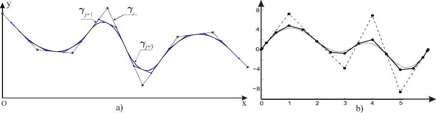
Fig. 1. a) Chaikin’s algorithm; b) The characteristic polygon lines of same curve ( n = 5)

Used in computer graphics for the construction of curves and surfaces, the famous Chaikin’s algorithm is a special case of such transformation (the previous transformation hereinafter will be called the generalized Chaikin’s algorithm). According to Chaikin’s algorithm [1], which is also called the "cutting corners" algorithm, the transition from a polygon line Yj to a polygon line Yj ₊₁ with vvertices c j ₊₁ , ₁ , c j ₊₁ , ₂ ,..., c j ₊₁ ,_{Nj +1} , Nj ₊₁ = 2 Nj — 2 is realized as follows (Fig. la)):

I,3

c j + 1 , 2 i- 1     4 c j,i + 4 c j,i + 1; c j + 1 , 2 i    4 c j,i + 4 c j + 1 ,i +1, i    ¹ , ² , . . . , ^Nj    ¹ .       ( d )

Equations (4) can be represented in a matrix form. Consider the matrix C T = (c j, ₁ ,..., c j,_Nj ) . Then (4) will turn to C j ₊₁ = P j ₊₁C j, where P j ₊₁ is the matrix from lemma 2 for n = 2.

Since supp фj,k = [ k ; k + n T¹ ] , then for t G [ S ; s j ] we get r j ( t ) = ^ Фj,k ( t )c j,k•

Therefore, if c j,_-n = ■■■ = c j,l, l >  0 , then r j ( t ) = c j,_-n, t G [0; l + j ¹ ] • Similarly, if c j, 2 j a ( n +1) -l = ■■■ = c j, 2 j a ( n +1) - 1 , l > n + 1 , th en r j ( t ) = c j, 2 j a ( n +1) - 1 , t G [ a ( n + 1) — l + j ¹; a ( n + 1)]. Figure 1 b) shows the characteristic polygon lines of same curve.

Now consider a surfaces with the parametric representation

2 j a ( n +1) - 1 2 ^k e ( m +1) - 1

r j,k ⁽ u^,v ) =    ^      ^    ^c jS фj,i ⁽ u ) фк,₈ ⁽ v ) ^{,u G [0}; ^{a (} n + ^{1)] ,v G [0}; ^{e (} m + ^1)] Л^

i=-n     s=-m where cjk = xjki + yj,kj + zjkk. As it is known, a polyhedron with vertices cj,k is called i,s i,s i,s i,s                                                                                          i,s the characteristic polyhedron of the surface. If we introduce the matrices Xj,k = (Xjk),

Yj,k = (yjS), Zj,k = (zjk) then the vector function rj,k can be represented as r j,k (u,v) = Ф j (u )Xj,k Ф k (v) Ti + Ф j (u )Yj,k Ф k (v) Tj + Ф j (u )Zj,k Ф k (v) Tk, he. the coordinates of this vector function belong to Vj 0 Vk.

Consider the following transformation of the characteristic polyhedron. Apply the generalized Chaikin’s algorithm to the polygon lines with vertices c j_s, s = —m, —m + 1 ,..., 2 ^k в ( m + 1) — 1 . The result is a set of vertices b j_s, s = —m, —m + 1 ,..., 2 ^{k +1} в ( m + 1) — 1. Next we apply the generalized Chaikin’s algorithm to the polygon lines with vertices b j _s, i = —n, —n + 1 ,..., 2 ^{j +1} a ( n + 1) — 1. These transformations can be reduced to the transformation of the matrix rows and columns. X j,k, Y j,k, Z j,_k.

X j +1 ,k +1 = P j +1X jk P T +1 , Y j +1 ,k +1 = P j +1Y j,k P T ₊₁ , Z j _+v+1 = P j +1Z j,k P T ₊₁

It’s clear that this transformation is a special case of transformation (2). As above, the characteristic polyhedron of the surface changes (condences) under these transformations, but the surface itself doesn’t.

3.    Mathematical Modelling of the Manufactureof Complex-Shaped Shells Out of Fiber Composite Materials

In practice, the complex surface of the mandrel for the future fiber composite product, is originally defined by its point frame, which is a result of the pattern-lofting method, based on the desired characteristics. The frame points may be used as the vertices of the mandrel’s characteristic polyhedron, therefore the mandrel can be defined by the parametric representation (5). The basic methods for producing the constructions out of the fiber composite materials (CM) are two related ones: filament winding, when the strip made of CM is laid out on the outstretched surface, and laying out. The automatic lay out is carried out in accordance with the program for moving the head of laying out machine (Fig. 2 a). To eliminate the gaping layers of tape to be laid on the mandrel the laying is normally accompanied with non-rigid roller pressing (Fig. 2 b) (the pictures are taken from [10]). Laying the tape on the mandrel can be modeled with a smooth

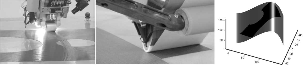
a)                                             b)                                        c)

Fig. 2. Simulation of the variable width tape on the surface

mapping of the rectangular area in three-dimensional Euclidean space (Fig. 2 c). If Y : r( s ) = r j,k ( uA ( s ) , vA ( s )) , s G [0; L ] is a parametric representation of the curve ( s is a variable arc length of the curve), which is where the tape is laying out (the reinforcement curve), then it determines the semigeodesic coordinate system [8] ( s,5 ) , s G [0; L ] , 5 G [ — d ; d ] ( d is the maximum width of the tape) on the surface. The result is a coordinate mapping F г : ( s, 5 ) ^ ( u ( s, 5 ) , v ( s, 5 )). It’s possible now to simulate the tape of variable width on the mandrel using the mapping w( s, 5 ) = r j,k о F _г о H ( s,5 ) , ( s, 5 ) G K = [0; L ] x [ — d ; d ] , where H is the local homeomorphism defining the width variation of the tape. In [4] it’s defined as follows: H ( s, 5 ) = ( s, —a 1( s ) + ( a 1( s ) + a ₂( s ))22+ d ) , — d < ai ( s ) < d, a 1( s ) + a ₂( s ) >  0 , Vs G [0; L ]. Unfortunately, the coordinate mapping F г can not be written explicitly, but it can be approximated with any accuracy with explicitly defined mappings of the desired smoothness [4]. In this paper, for an approximation of the coordinate mapping we’ll use the mapping F : ( s,5 ) ^ ( U ( s,5 ) , V ( s, 5 )). defined by equation

( U ⁽ s, ⁵ ) ) _ ( ^un,v )   ।    ^{5   5}v   ( ^un,v +1    ^un,v )   । s   sn   ( un +1 ,v   ^un,v

V ⁽ s, ⁵ )        vn,v     ⁵v +1 ^{— 5}v   vn,v +1 ^— vn,v     sn +1 ^{— s}n  vn +1 V ^— vn,v

+

5 — 5v   s — sn

¹ v +1 ^{— 5}v ^sn +1 ^{— s}n

(un+1 ,v +1 — un+1 ,v — un,v +1 + unv vn+1 ,v +1 — vn+1 ,v — vn,v+1 + vn,v s G [sn ; sn+1], 5 G [5v ; 5v+1 ], where — d = 5-I < 5-I+1 < • • • < 5I- 1 < 5I = d, 0 = sо < s 1 < • • • < sJ = L are nets on the segments [ — d; d] and [0; L] respectively. The values of un,v and vn,v can be found out of the solution of systems of differential equations that define the geodesic coordinate on the surface passing through the points (uA (sn), vA (sn)) of the reinforcing curve perpendicular to it [4]. It is easy to see that if the functions u(s,5) и v(s, 5) are continuous and A = max(V(sn - sn+1)2 + (5v - 5v+1)2)- theu ||u — U||c(к)    < ш(u, A),

η,ν

|v — V||c ( к ) < ш ( v, A), where ш ( f, A) is the modulus of continuity of f. The example of modelling of the variable width tape on the surface is shown in Fig. 2.

It should be noted that the automated laying out of the fibers or winding of the unidirectional fiber tape assumes that the width of the tape should not exceed the value at which for all ( s, 5 ) G K | tg 0( s, 5 ) | < p , where 0( s, 5 ) is the geodesic deviation angle [8] of the curve w ( s, 5 ) , s G [0; L ]. which the thread is laying out along, p is the coefficient of sliding friction of the surface and filament materials. In this case, the the threads of the tape will be in equilibrium.

When laying tape on the mandrel the shape of the surface changes, because the tape has a non-zero thickness. This fact can be taken into account by tuning the characteristic polyhedron of the surface (as a consequence there is a local change in the shape of the surface). For more accurate accounting there must be a large number of vertices of the polyhedron. We’ll get the reconstruction of the polyhedron with the help of the generalized Chaikin’s algorithm. Fig. 3 a) shows the vertices of the characteristic polyhedron defining the fan blade. Fig. 3 b) shows the result of the generalized Chaikin’s algorithm to a given characteristic polyhedron of the blade, which does not change the blade. Fig. 3 c) shows the blade itself.

The blade operates under the high-tense state. The main loads are centrifugal ones as a result of high rotation speed (around 4000 rev / min). In addition, the blade is under

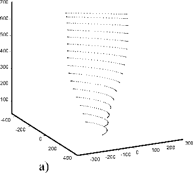
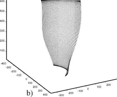
Fig. 3. The characteristic polyhedra of the fan blade a), b) and the blade itself c)

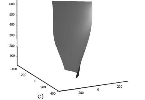
the aerodynamic loads of the air flow which cause its bending moments and torsion. To counter the stretching due to centrifugal loads and bending the blade must be reinforced with carbon fibers directed along the axis Z (the axis passing through the engine axis of rotation and perpendicular to it. In Fig. 3 it’s a the vertical axis). The main requirement for torsional resistance is the torsional stiffness of the blade, which requires reinforcement in the directions ± 45 ° to the axis Z. The calculations also show that there are high shear interlayer loads, which in some parts of the piece are above the limit for existing domestic aircraft carbon composites. Basically, this problem is solved by material science and technological developments. However, to avoid additional shear interlayer loads, the reinforcing fibers must be placed along the geodesic lines. Used geodesic lines require the surface of class C ². Therefore, iii formula (5) n = m = 3 , a = в = 1 •

Converting the surface after the tape laying is carried out as follows. Let the surface of the mandrel be defined by parametric representation (5) and E j,k = { c jk} j —n^ ( ^{m +1)} - ¹ are the vertices of its characteristic polyhedron. Choosing natural N we apply the generalized Chaikin’s algorithm to this polyhedron and obtain polyhedron ^E j ₊ Nk ₊ n = ^{ c ^{j + N,k + N}} ² — —^——"т, 2 + ⁽ m ⁺¹⁾ - ¹ (wavelet recovery):

^E j,k

P j + 1 , P k +q _v          P j +2 , P k +2

'          ^ ^E j +1 ,k +1      '          ^ • •

P j + N , P k + N

E j + N,k + N

Let ⁽ u, v ) G ^[2 j + n ; 2 j + n ^] ^ ^[2 k + n ; 2 П + n ^] Tlien

νη rj + N,k+N (u,v)= ^2 52 cй^+NФз+N,i (u) Фк+N,s (v) • i—v—n s—n~m

The vertices {cj+N,k+NY;''1,,          of the conversion polyhedron of the surface are defined i,s                 iv n, s ii 11m as follows b3 +Nk+N

cj+N,k+N cjAk+N + f (6) he

if ( u,v ) G F ( K ); if ( u,v ) G F ( K )

i = v — n,... ,v ; s = n — m, • • • ,П,

(s,6) = F 1(u,v), where e is a unit vector normal tо the surface at the point (u, v). f (5), 6 G [ — |; d] is a smoothing function and h is a tape thickness. In this example the smoothing function was chosen as follows:

f ( 5 ) =

1 ,

_ ( 5- A)² e σ

_ ( 5 +A)² e ^σ

If 5 e [ - △ ; △ ];

if 5 e [ △ ; 2];     0 <   △ 0 .

if 5 e [ - d ; - △ ] ,

After laying of the first layer is performed the smoothing of the surface is obtained by formulas (3) (wavelet decomposition):

^ j,k '             ^ j + 1 ,k +1 ^

^A j ± N , ^A k ± N

^ j + N,k + N ■

The result of the algorithm is shown in Fig. 4. Further we simulate the second layer, etc.

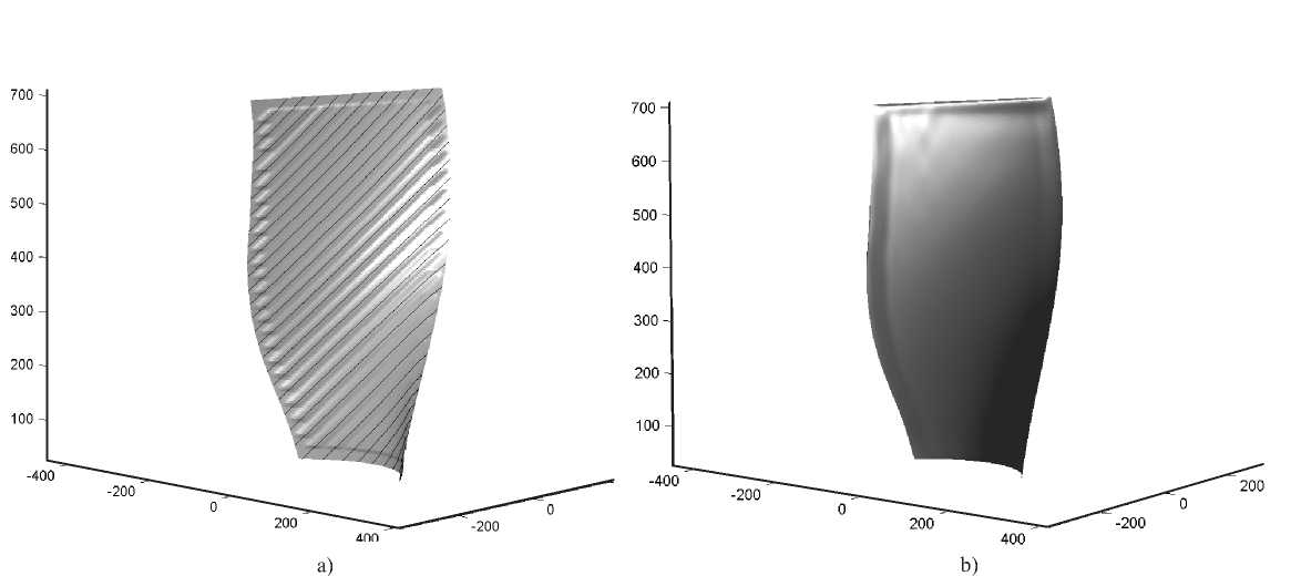
Fig. 4. a) Simulation of the first layer laying; b) Smoothing the surface

As noted above, the laying out is performed using a special roller in accordance with the moving program of the laying out head. In conclusion, we’ll present the trajectory of the pressure roller. Its position in space can be described by two coordinates of its points A and В on the roller’s axis (Fig. 5 a). Then the position of the roller at any moment can be described by the vector functions r A ( s ) = w ( s, — d ) + p e о F ( s, — d ) and r_B ( s ) = w ( s, d ) + p e о F ( s, d ). wlicre p is the roller's radius and e ( u,v ) = ,^r u ^{( u,v} ) * ^r V ^{( u,v} ), . B                  ^, 2                       ^, 2                                                                         ^,           | r U ( u,v ) x r V ( u,v ) |

Analysis of the equilibrium of some fibers of the tape is shown on Fig. 5 b).

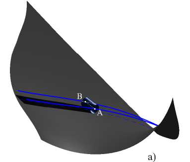
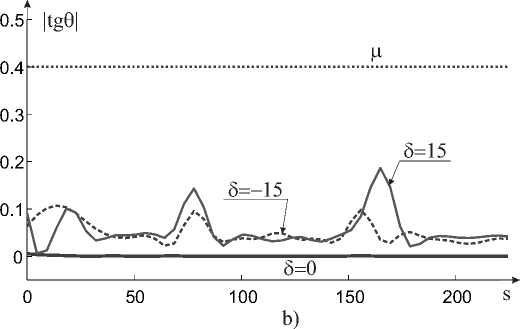
Fig. 5. a) The trajectory of the laying out machine head’s pressing roller; b) Analysis of the equilibrium of some fibers of the tape

Conclusion

In this paper, the semi-orthogonal wavelet systems are used in the mathematical and computer modelling of the manufacture of complex-shaped shells made of fibrous composite materials. As an example the producing of the fan blade by the laying out method is simulated. However, these results can be used in the development of CAD/CAM/CAE-system for the manufacturing of the shells made of fibrous composite materials by any of related process: laying out and winding.