Thermodynamic trade-off of control performance in quantum fuzzy inference: port-controlled Hamiltonian systems applications

Author: Barchatova Irina
Journal: Сетевое научное издание «Системный анализ в науке и образовании» @journal-sanse
Article in issue: 3, 2014.
Free access
As example of control object model port-controlled Hamiltonian systems are consider. Port-controlled Hamiltonian systems are the generalization of conventional Hamiltonian systems. They can describe not only mechanical systems but also a broad class of physical systems including passive electro-mechanical systems, hydraulic, gas, mechanical systems with non-holonomic constraints and their combinations. Port-controlled Hamiltonian systems describe, in a modular, network-like way, the interconnection of physical systems using the transfer of energy and entropy as the unifying concept. Thermodynamic trade - off between stability, controllability and robustness for described class of systems is introduced. Simulation of robust control based on quantum fuzzy inference is considered.
Thermodynamic trade - off, stability, robustness, controllability, quantum fuzzy inference
Short address: https://sciup.org/14123248
IDR: 14123248
Термодинамическое распределение качеств управления в квантовом нечетком выводе: применение в порт-гамильтоновых системах
Рассматривается объект управления модель порт-Гамильтоновых систем, которые являются обобщением всех Гамильтоновых систем с разнородной структурой. Данные объекты управления могут быть описаны не только механическими системами, но охватывают более широкий класс физических систем, например, пассивные электро-механические, гидравлические, газовые, механические системы с неголономными связями и др. Порт-Гамильтоновы системы, как динамические объекты, могут быть описаны в виде взаимосвязанных модулей или сетей, представляющих собой физические системы с переносом энергии и энтропии и представляют собой единую концепцию описания их динамического поведения. Для данных систем рассматривается термодинамическое распределение качеств управления: управляемость, устойчивость и робастность. Результаты моделирования робастного управления такими системами рассмотрено на основе квантового нечеткого вывода.
Text of the scientific article Thermodynamic trade-off of control performance in quantum fuzzy inference: port-controlled Hamiltonian systems applications
Introduction: Control object model and energy based hybrid controller
In control engineering, dissipative theory, which encompasses passivity theory, provides a fundamental framework for the analysis and control design of dynamical systems using an input-output system descrip- tion based on system energy related considerations. Energy is a concept that underlies the understanding of all physical phenomena and is a measure of the ability of a dynamical system to produce changes (motion) in its own system state as well as changes in the system states of its surroundings. The notion of energy here refers to abstract energy notions for which a physical system energy interpretation is not necessary. The dissipation hypothesis on dynamical systems results in a fundamental constraint on their dynamic behavior, wherein a dissipative dynamical system can only deliver a fraction of its energy to its surroundings and can only store a fraction of the work done to it.
Thus, dissipative theory provides a powerful framework for the analysis and control design of dynamical systems based on generalized energy considerations by exploiting the notion that numerous physical systems have certain input-output properties related to conservation, dissipation, and transport of energy. Such conservation laws are prevalent in dynamical systems such as mechanical systems, fluid systems, electromechanical systems, electrical systems, combustion systems, structural vibration systems, biological systems, physiological systems, power systems, telecommunications systems, and economic systems, to cite but a few examples. Energy-based control for Euler-Lagrange dynamical systems and Hamiltonian dynamical systems based on passivity notions has received considerable attention [1].
This controller design technique achieves system stabilization by shaping the energy of the closed-loop system which involves the physical system energy and the controller emulated energy. Specifically, energy shaping is achieved by modifying the system potential energy in such a way so that the shaped potential energy function for the closed-loop system possesses a unique global minimum at a desired equilibrium point. Next, damping is injected via feedback control modifying the system dissipation to guarantee asymptotic stability of the closed-loop system.
A central feature of this energy-based stabilization approach is that the Lagrangian system form is preserved at the closed-loop system level. Furthermore, the control action has a clear physical energy interpretation, wherein the total energy of the closed-loop Euler-Lagrange system corresponds to the difference between the physical system energy and the emulated energy supplied by the controller [2].
A novel energy dissipating hybrid control framework was developed for Euler-Lagrangian, port-controlled Hamiltonian systems (PCHS) [3], and lossless dynamical systems. The fixed-order, energy based hybrid controller is a hybrid controller that emulates a hybrid Hamiltonian dynamical system and exploits the feature that the states of the dynamic controller may be reset to enhance the overall energy dissipation in the closed-loop system. An important feature of the hybrid controller is that its Hamiltonian structure can be associated with a kinetic and potential energy function. In a mechanical Euler-Lagrange system, positions typically correspond to elastic deformations, which contribute to the potential energy of the system, whereas velocities typically correspond to moments, which contribute to the kinetic energy of the system.
On the other hand, while an energy-based hybrid controller has dynamical states that emulate the motion of a physical Hamiltonian system, these states only “exist” as numerical representations inside the processor. Consequently, while one can associate an emulated energy with these states, this energy is merely a mathematical construct and does not correspond to any physical form of energy.
The central mathematical object of the formulation is what is called a Dirac structure [3], which encodes the detailed connecting network information. A main feature of the formalism is that the interconnection of Hamiltonian subsystems using a Dirac’s structure yields again a Hamiltonian system.
A PCHS model encodes the detailed energy transfer and storage in the system, and is thus suitable for control schemes based on, and easily interpretable in terms of, the physics of the system.
Port-controlled Hamiltonian Systems (PCHS)
A time-varying PCHS with dissipation is a system of the form:
Г / х / x-i d H ( x , t )T / x z XT d н ( X, t ) T
X = 1 J ( X, t)-R ( X, t )|-----—’—gr g ( X, t) u, y = g ( X, t) ----------. (1)
оx дx with a Hamiltonian H(x, t)e R, u,y E Rm, x E Rn, a skew symmetric matrix J (x, t), i.e. J = —JT holds, and a positive semi-definite symmetric matrix R (x, t)> 0 are the interconnection and damping matrices, respectively. A PCHS is passive [3] if
'd H ( x , t )Y
< d x j
, . dH ( x , t )
R ( x , t )---------- dt .
V 7 dx
J u T ydt = H ( x, t ) — H ( x ,0 ) + J 0 0
The essential fact about PCHS’s is that, in a given sense, power preserving interconnection of several PCHS yields a Hamiltonian system (with or without ports). The rigorous result is that interconnection of PCHS by means of what is called a Dirac structure yields an implicit PCHS.
Remark . PCHS naturally arise from a network modeling of physical systems without dissipative elements. Recall that a PCHS is defined by a state space manifold X endowed with a triple ( J, g , H ) . The pair ( J ( x ) , g ( x ) ) , x e X , captures the interconnection structure of the system, with g ( x ) modeling in particular the ports of the system. Independently from the interconnection structure, the function H :X ^ R defines the total stored energy of the system. Furthermore, PCHS are intrinsically modular in the sense that a powerconserving interconnection of a number of PCHS again defines a PCHS, with its overall interconnection structure determined by the interconnection structures of the composing individual systems together with their power-conserving interconnection, and the Hamiltonian just the sum of the individual Hamiltonians.
A basic property of PCHS is the energy balancing property
dH dt
(x, t)
< u T ( t ) y ( t ) showing that a
PCHS is passive if the Hamiltonian H is bounded from below. Physically this corresponds to the fact that the internal interconnection structure is power-conserving (because of skew-symmetry of J ( x ) ), while u and
У are the power-variables of the ports defined by g ( x) ; and thus uT (t) y (t) is the externally supplied pow- er.
More precise results about the possibility of obtaining invariant manifolds expressing the controller variables in terms of the variables of the system can be formulated if both system and controller are PCHS. Let us consider the system
S : x = [ J ( x, t ) — R ( x, t ) ]---- ^ ,
+ g ( x , t ) u,
y = g ( x , t ) T
d H ( x, t ) T
• Г / x dH (5, t)T z X z XT dH (^, t)T
S c : ^ = [ J c ( ^ , t ) — R c ( ^ , t ) ]----—---- + g c ( 5 , t ) u c , У с = g c ( ^ , t ) ----52^'
With the power preserving, standard negative feedback interconnection, u = — yc , uc = y , one gets
( H
_ ( J (x) — R (x) — g (x) gTc (^)) dx
) J 5 Hd ’
I d 5 J
gc (^)gT (x) Jc (x) — Rc (x.
where H d ( x , 5 ) = H ( x ) + H c ( ^ ) . Let’s look next for invariant manifolds of the form:
Ck (x,5)=F (x)—5+K'
Condition CK = 0 yields that


' J - R
V g c g T
H)
—ggc j dX
= 0.
J - R c J ^ HA,
I '- J
Since we want to keep the freedom to choose H , we demand that the above equation is satisfied on C for every Hamiltonian, i.e. we impose F on the following system of partial differential equations (PDE’s):
/ / x T ^dF | V d x J
' J - R
„ _ T
V g c g
- gg C
J c - R c
= 0.
Functions C K ( x,£) such, that satisfies the above PDE on C k (V) = 0 are called Casimir functions . They are invariants associated to the structure of the system ( J , R , g , Jc , Rc , gc ) , independently of the Hamiltonian function.
The PDE for F has solution if and only if ( iff) , on C K ( X , £ ) ,
(dF Y a F 0F (FF Y T
(c 1 ) I I J1T = J c ; (C 2 ) R = 0; (C 3 ) R c = 0; (C 4 ) I I J = g c gT .
V dx Jox dx V dx J
Remark . Conditions (C 2 ) and (C 3 ) are easy to understand: essentially, no Casimir functions exist in presence of dissipation. Given the structure of the PDE, Rc = 0 is unavoidable, but we can have an effective R = 0 just by demanding that the coordinates on which the Casimir depends do not have dissipation, and hence condition (C 2 ). If the proceeding conditions are fulfilled, an easy computation shows that the dynamics on is given by
x = ( J (x)-R (x))
d Hd dx
with Hd = H (x) + Hc (F (x) + K).
Notice also, that due to condition (C 2 ),
R(x>дН"(F(x) + K) = R(x)|F^Ht(F(x) + K) = 0 • dx dx dx
= 0
so we can say that dissipation is only admissible for those coordinates which do not require energy shaping. Remark . A pseudo-Hamiltonian dissipative dynamic system are described as
x = M(x)—, x G R”, 5x where M (x) is an H x ” matrix with entries as Cr function on R”/ {0}, called the structure matrix. H g Cr (R ”) is the Hamiltonian function of the system. Then under the regularity assumption, we have a unique decomposition of M (x) as following: M(x) = J(x) - R (x) + T(x). A controlled dissipative pseudoHamiltonian system or PCHS ifT (x ) = 0. The generalization, provided by the concept of pseudoHamiltonian system is to allow T (x)^ 0. The motivation for this generalization lies on the following two points.
First of all, converting an affine nonlinear system into a port-controlled Hamiltonian system directly is difficult. But, roughly speaking, almost all the affine nonlinear systems can be converted to the pseudoHamiltonian systems. Moreover, almost all the functions can be the Hamiltonian function for a given nonlinear system. So this approach can cover a very large class of systems. Secondly, some conditions are known to convert a pseudo-Hamiltonian system to the PCHS via feedback.
Then a two step realization can be proposed as:
Dynamic system ^ pseudo-Hamiltonian system ^ PCHS, and the well established theory for PCHS may be used for a large class of control systems.
Remark . Variable structure systems (VSS) [or sliding mode control] are piecewise smooth systems, i.e. systems evolving under a given set of regular differential equations until an event, determined either by an external clock or by an internal transition, makes the system evolve under another set of equations; in particular, this kind of behavior can occur periodically, and might give rise to very complicated dynamical features. VSS appear in a variety of engineering applications, where the non-smoothness is introduced either by physical events, such as impacts or switching, or by a control action, as in hybrid or sliding mode control . Typical fields of application are rigid body mechanics with impacts or switching circuits in power electronics. Let VSS system be described in explicit port Hamiltonian form
X = Г J ( 5 , X ) - R ( 5 , X ) 1---+ g ( 5 , X ) U ,
L J dx where s is a (multi)-index, with values on a finite, discrete set, enumerating the different structure topologies. For notational simplicity, we will assume that we have a single index (corresponding to a single switch, or a set of switches with a single degree of freedom) and that 5 G {0,1} . Hence, we have two possible PCHS dynamics, which we denote as
5 = 0 ^ X = [ Jo ( 5, X)- Ro ( 5, X
dH (x)
5 = 1 ^ X = [ J (5, X )- R, (5, X
J dX
dH ( x ) dx
+ g 0 ( 5 , X ) u ,
+ g j ( 5 , X ) U .
Note that controlling the system means choosing the value s of as a function of the state variables and that u is, in most cases, just a constant external input. If the system (1) has a semi positive definite Hamiltonian, i.e.,H ( x , t )>H(X,0) = 0, and ^- < 0 holds. Then the input-output mapping u H y becomes passive d t and consequently the feedback u =
with a positive definite matrix C ( X , t ) > £ l > 0 renders ( U , y ) ^ 0 .
Suppose moreover that the system is periodic and zero-state detectable and that H is positive definite and decrescent. Then the feedback (2) renders the system uniformly asymptotically stable.
/ _ X T i T fdH )'
Let the target signal h I----I and take its integrated value
V dx J
t z = J h T ( x , t)
^d H ( x , t )
V d X
T dt
that involved into the stabilizing controller and the feedback (2).
Here z g R k and h g R n x k . Let us define the extended state Xe : = ( X , z ) . Then we readily find that the dynamics of the whole system with the extended state x is described by a PCHS:
where
xe ={ Je ( x, t )-Re ( x, t )} ^H£x’ t ) +
g e ( x , t ) u,
t dH (x, t )T У = ge (x, t) ; ’ , dx
Je =
|
J - h л |
Г R 0 ) |
Г g ^ |
||
|
h T 0 ? |
, R e = |
V 0 0 J |
, g e = |
V 0 j |
.
V
Stabilization of this system implies integral control of the original. A trajectory tracking problem and error control may to convert into a stabilization problem.
Remark . More precisely, let us consider a general nonlinear system x = ф ( x,u , t ) , x ( 0 ) = x 0 and assume that the desired trajectory of the state x ( t ) on the time interval t e [ 0, ^ ) is given by xd ( t ) and that it is realizable, that is, there exists an admissible input ud ( t ) such that x d = ф ( xd , ud , t ) . The objective is to achieve the following goal: || x ( t ) - xd ( t )||^ 0 as t ^ 0.
For this problem, we usually calculate the dynamics of the tracking error x : = x - xd as x = x - x d = ф ( x , u , t ) - x d = ^ ( x + x d, u , t ) - xd
^ ( x , u , t )
and try to stabilize this system. Here the error system (5) sometimes becomes more complicated than the original x = ^ ( x , u , t ) , x ( 0 ) = x 0 and hard to be stabilized. In order to attain the objective ||x ( t ) - xd ( t )|| ^ 0 as t ^ 0, however, the error system does not need to have the form (5) and we can consider an error system in a more general form as given in the following definition.
A system described by
x = ф(x,u, t), x (0) = ф(x0)
with a smooth function ф is said to be an error system of x = ф ( x , u , t ) , x ( 0 ) = x 0 with respect to the desired
trajectory xd (t) if x (t) = 0 О x(t) = xd (t) holds for all
u .
For the definition of the error system, it is obvious that stabilization (settling the state at the origin) of the error system implies the tracking control of the original system. It was proposed a procedure to realize an error system of a given PCHS (1) by another PCHS via the generalized canonical transformation:
x =Ф(x,t), H = H(x,t) + U(x,t), y = y + a(x,t), u = u + в(x,t),
which preserves the structure of port-controlled Hamiltonian systems with dissipation, that is, the system into an appropriate Hamiltonian system in such a way that the transformed system
x =[ J (x, t)-R (x, t )]SH(x, t)T
+ g (x, t) u,
y = g (x, t )T
dH (x, t) dx
satisfies x (t) = 0 О x (t) = xd (t).
Hamiltonian has its minimum value on the desired trajectory, that is,
(H + U)(x,t) > (H + U)(xd (t),t) = 0, Vt e [0,^), since the new Hamiltonian function plays the role of the Lyapunov function when we stabilize the error system.
Thus, if the state trajectory X ( t ) of the original system (1) can be distinguished by x 0 and
y (t ) = y (t) + a( x, t)
in the sense that X0 = Xd (0), y (t ) = 0, Vt e[0, w)^ X (t ) = Xd (t) Vt e[0, w) with storage function H as
L x5( h + mem s( h + и V )
( J - R ) \ / --5 ----)- + gp
d ( x , t ) d x d x
^ 0,
- 1
then the constructed PCHS is an error system of the original one (1).
Thus we can achieve the tracking control via stabilization and the feedback (2).
Therefore, using the generalized canonical transformation, we can change the property of the system without changing the intrinsic passive property. Indeed if a given system fails to satisfy the stabilizability conditions by the feedback (2): positive definiteness of the Hamiltonian function and zero-state detectability, then still we may be able to transform the system into an appropriate Hamiltonian system which can be stabilized by the feedback (2).
Control performance: Thermodynamic trade-off and interrelations between stability, controllability and robustness
According to Figure 1, one of the main tasks of designing an intelligent control systems (ICS) consists in providing that the developed (chosen) structure possesses the required level of control quality and robustness (supports the required indices of reliability and accuracy of control under the conditions of information uncertainty).
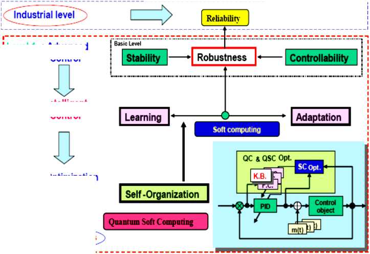
Figure 1. Performance and interrelations between of control quality criteria
Level 1 : Advanced Control
Level 2 : Intelligent Control
Level 3 : Optimization byQSC
Note that one of the most important and hard-to-solve problems of designing ICS’s is the design of robust KB that allow the ICS to operate under the conditions of information uncertainty. The core of technique for designing robust KB of FC’s is generated by new types of computing and simulation processes.
Remark. We are witnessing a rapidly growing interest in the field of advanced computational intelligence, a "soft computing" technique. Soft computing integrates fuzzy logic, neural networks, evolutionary computation, and chaos. Soft computing is the most important technology available for designing intelligent systems and control. The difficulties of fuzzy logic involve acquiring knowledge from experts and finding knowledge for unknown tasks. This is related to design problems in constructing fuzzy rules. Fuzzy neural networks (FNN’s) and genetic algorithms (GA’s) are attracting attention for their potential in raising the efficiency of knowledge finding and acquisition. Combining the technologies of fuzzy logic, FNN’s and GA’s, i.e., soft computing techniques will have a tremendous impact on the fields of intelligent systems and control design.
To explain the apparent success of soft computing, we must determine the basic capabilities of different soft computing frameworks.
Recently, the application of ICS structures based on new types of computations (such as soft, quantum, etc., computing) has drawn the ever-increasing attention of researchers. Numerous investigations conducted have shown that they possess the following points of favor: retain the main advantages of conventional automatic control systems (such as stability, controllability, observable-ability, etc.); have an optimal (from the point of view of a given control objective performance) KB, as well as a possibility of correcting with learning it and adapting it to the changing control situation; guarantee the attainability of the required control quality based on the designed KB; are open systems, i.e., they allow one to introduce an additional objective performance for control and constraints on the characteristics of the control process.
One of the main problems of modern control theory is to develop and design automatic control systems that meet the three main requirements: stability , controllability , and robustness . The listed quality criteria ensure the required accuracy of control and reliability of operation of the controlled object under the conditions of incomplete information about the external perturbations and under noise in the measurement and control channels, uncertainty in either the structure or parameters of the control object, or under limited possibility of a formalized description of the control goal.
Therefore, in practice of advanced control systems main sources of unpredicted control situations are as following:
-
1. Control object
Type of unstable dynamic behavior
-
- Local unstable
-
- Global unstable
-
- Partial unstable on generalized coordinate and non-linear braces.
Time-dependent random structure or parametric excitations
Type of model description
-
- Mathematical model
-
- Physical model
-
- Partial mathematical and fuzzy physical model.
-
2. External random excitations
-
3. Measurement system
-
4. Different types of reference signals
-
5. Different types of traditional controllers
Different probability density functions
Time-dependent probability functions
Sensor noise
Time delay
Random time delay with sensor noise
This problem is solved in three stages as following:
-
(1) The characteristics of stability of the controlled plant are determined for fixed conditions of its operation in the external environment;
-
(2) A control law is formed that provides the stability of operation of the controlled plant for a given accuracy of control (according to a given criteria of the optimal control);
-
(3) The sensitivity and robustness of the dynamic behavior of the controlled plant are tested for various classes of random perturbations and noise.
These design stages are considered by modern control theory as relatively independent. The main problem of designing automatic control systems is to determine an optimal interaction between these three quality indices of control performance. For robust structures of automatic control systems, a physical control principle can be proven that allows one to establish in an analytic form the correspondence between the required level of stability, controllability, and robustness of the control. This allows one to determine the required intelligence level of the automatic control system depending on the complexity of the particular control problem.
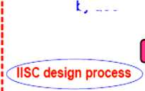
Let us consider in short the main physical principles of an energy-based control processes that allow one to establish the interrelation between the qualitative dynamic characteristics of the controlled plant and the actuator of the automatic control system: stability, controllability, and robustness of control. For this purpose, we are employing the informational and thermodynamic approaches that join by a homogeneous condition the criteria of dynamic stability (the Lyapunov’s function), controllability, and robustness.
Example: Thermodynamics trade-off between stability, controllability, and robustness. Consider a dynamic controlled plant given (in a general form of (1)) by the equation dq = ^(q,S(t),t,u,£(t)), u = f(q,qd,t) , (8)
where q is the vector of generalized coordinates describing the dynamics of the controlled plant; S is the generalized entropy of dynamic system (3); u is the control force (the output of the actuator of the automatic control system); qd (t) is reference signal, £(t) is random disturbance and t is the time. The necessary and sufficient conditions of asymptotic stability of dynamic system (1) with £(t) = 0 are determined by the physical constraints (for example, as for PCHS) on the form of the Lyapunov function, which possesses two important properties represented by the following conditions:
-
(I) This is a strictly positive function of generalized coordinates, i.e., V > 0 ;
-
(II) The complete derivative in time of the Lyapunov’s function is a non-positive function,
dV s o .
dt
In general case the Lagrangian dynamic system (8) is not lossless with corresponding outputs.
By conditions (I) and (II), as the generalized Lyapunov function, we take the function
n
V = 2 § q i + 2 S 2 •
where S = S p — S c is the production of entropy in the open system «control object + controller »; S p =* ( q - q - t ) is the production of entropy in the controlled plant; and Sc = Y ( e, t ) is the production of entropy in the controller (actuator of the automatic control system). It is possible to introduce the entropy characteristics in Eqs. (8) and (9) because of the scalar property of entropy as a function of time, S ( t ) .
Remark. It is worth noting that the presence of entropy production in (8) as a parameter (for example, entropy production term in dissipative process R ( x, S, t ) in Eq. (1)) reflects the dynamics of the behavior of the CO and results in a new class of substantially nonlinear dynamic automatic control systems. The choice of the minimum entropy production both in the control object and in the fuzzy PID controller as a fitness function in the GA allows one to obtain feasible robust control laws for the gains in the fuzzy PID controller.
The entropy production of a dynamic system is characterized uniquely by the parameters of the nonlinear dynamic automatic control system, which results in determination of an optimal selective trajectory from the set of possible trajectories in optimization problems. Thus, the first condition is fulfilled automatically. As- dV sume that the second condition < 0 holds.
dt
In this case, the complete derivative of the Lyapunov function (9) has the form dV = E qq + SS = E q^i (q, S, t, u)+(Scob tii
- S c ) ( S cob - S c ) .
Thus, taking into account (8) and the notation introduced above, we have dV dt Stability
= E qMq , >T V| , t , u ) + ( ^-y ) ( ^-y ) < о
z
Controllability
Robustness
Figure 2 show the role of developed thermodynamic trade-off in robust control design.
Relation (11) relates the stability, controllability, and robustness properties.
Remark . This approach was firstly presented in [4]. It was introduced the new physical measure of control quality (10) to complex non-linear controlled objects described as non-linear dissipative models. This physical measure of control quality is based on the physical law of minimum entropy production rate in ICS and in dynamic behavior of complex object. The problem of the minimum entropy production rate is equivalent with the associated problem of the maximum released mechanical work as the optimal solutions of corresponding Hamilton-Jacobi-Bellman equations. It has shown that the variational fixed-end problem of the maximum work W is equivalent to the variational fixed-end problem of the minimum entropy production . In this case both optimal solutions are equivalent for the dynamic control of complex systems and the principle of minimum of entropy production guarantee the maximal released mechanical work with intelligent operations. This new physical measure of control quality we using as fitness function of GA in optimal control system design.
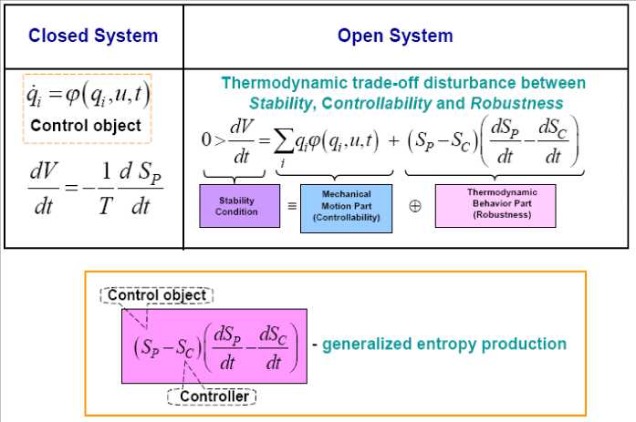
Figure 2. Physical law of intelligent control as background of IFICS design technology
In the case of PCHS (7) we have
dV dHi (xi, t) — \ —
— = E xi [ J* (x, t) - Ri (xi,S, t)]——+gi (x, t) u
^d t i dv ^X^
Stability Controllability
+ ( v-y ) ( ^-y ) < 0.
Robustness
In [2, 3] have studied something similar, what was called as «equipartition of energy».
Such state corresponds to the minimum of system entropy.
The introduction of physical criteria (the minimum entropy production rate) can guarantee the stability and robustness of control. This method differs from aforesaid design method in that a new intelligent global feedback in control system is introduced. The interrelation between the stability of CO (the Lyapunov function) and controllability (the entropy production rate) is used. The basic peculiarity of the given method is the necessity of model investigation for control object and the calculation of entropy production rate through the parameters of the developed model. The integration of joint systems of equations (the equations of mechanical model motion and the equations of entropy production rate) enable to use the result as the fitness function in GA as a new type of CI. Acceleration method of integration for these equations is described in [5].
Remark . The concept of an energy-based hybrid controller can be viewed from (8.16) also as a feedback control technique that exploits the coupling between a physical dynamical system and an energy-based controller to efficiently remove energy from the physical system. According to (8.15) we have
£ q^Xq, (V-Y), t, u )+(T-Y)(V-Y)s 0,
i or
£q№(q,(T-Y),t,u)<(Т-Г)(Г-ф) . (12)
z
Therefore, we have different possibilities for support inequalities in (12) as following:
-
(i) £qq< 0, (V>Y),(Y> V), SS > 0 ;
i
-
(ii) £ qq < 0, ( V
), (Y ), SS > 0; z
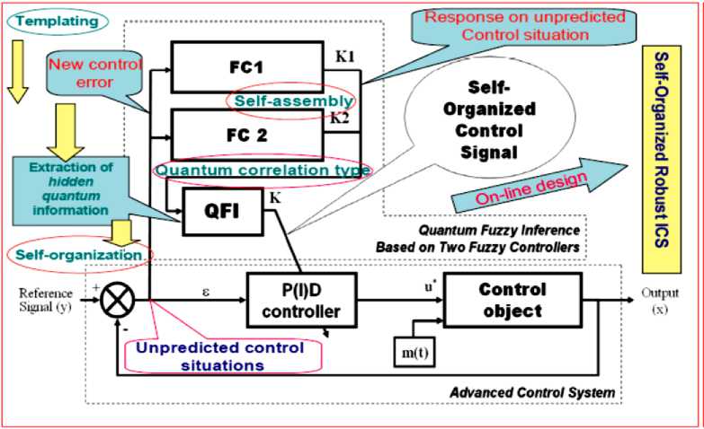
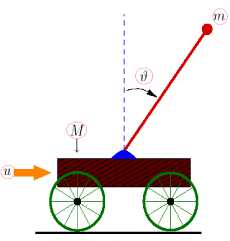
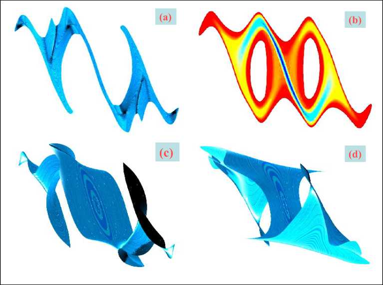
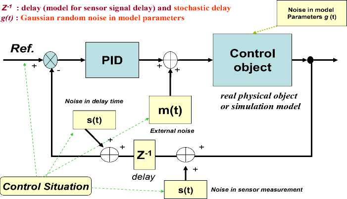
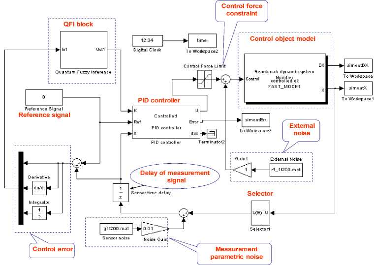
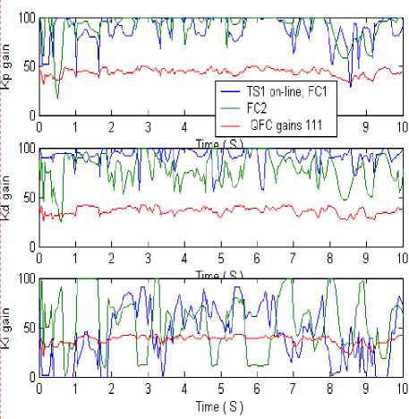
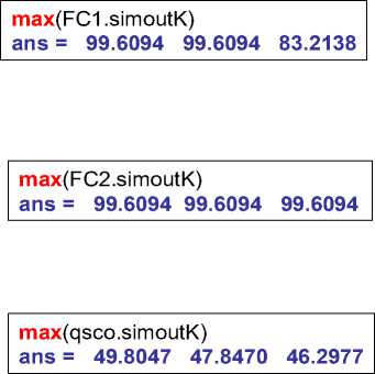
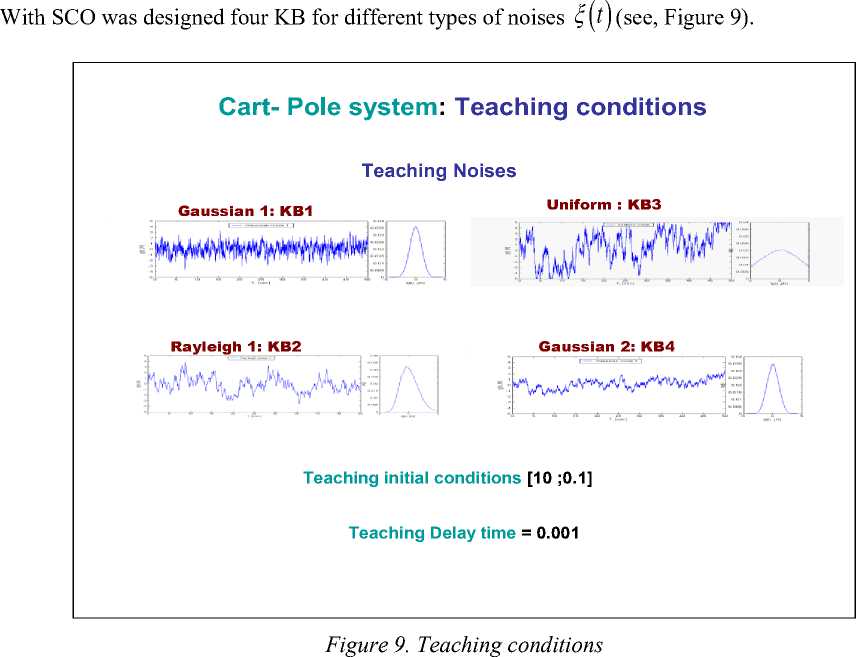
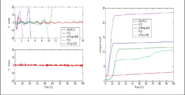
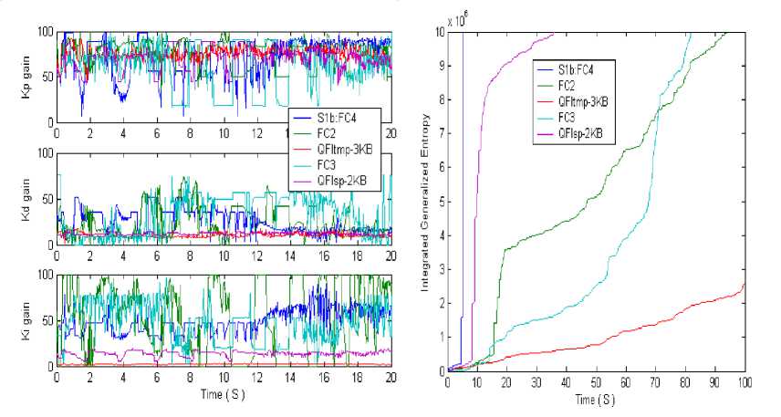
(iii)£qqi<0,(T These inequalities specifically, if a dissipative or lossless CO is at high energy level, and a lossless feedback controller at a low energy level is attached to it, then energy will generally tends to flow from the CO into the controller, decreasing the CO energy and increasing the controller energy. Emulated energy, and not physical energy, is accumulated by the controller. Conversely, if the attached controller is at a high energy level and a plant is at a low energy level, then energy can flow from the controller to the plant, since a controller can generate real, physical energy to effect the required energy flow. Hence, if and when the controller states coincide with a high emulated energy level, then it is possible reset these states to remove the emulated energy so that the emulated energy is not returned to the plant. In this case, the overall closed-loop system consisting of the plant and the controller possesses discontinuous flows since it combines logical switching with continuous dynamics, leading to impulsive differential equations. A continuous-time system in the feedback interconnection with the resetting controller is considering in [6]. Every time the emulated energy of the controller reaches its maximum, the states of the controller reset in such a way that the controller's emulated energy becomes zero. Alternatively, the controller states can be made reset every time the emulated energy is equal to the actual energy of the plant, enforcing the second law of thermodynamics that ensures that the energy flows from the more energetic system (the plant) to the less energetic system (the controller). The proof of asymptotic stability of the closed-loop system in this case requires the non-trivial extension of the hybrid invariance principle, which in turn is a very recent extension of the classical Barbashin-Krasovskii invariant set theorem. The subtlety here is that the resetting set is not a closed set and as such a new transversality condition involving higher-order Lie derivatives is needed. A system theoretic foundation for thermodynamics is developed in [2]. Main goal of robust intelligent control is support of optimal trade-off between stability, controllability and robustness with thermodynamic relation as (10) or (11) as thermodynamically stabilizing compensator. The resetting set is thus defined to be the set of all points in the closed-loop state space that correspond to decreasing controller emulated energy. By resetting the controller states, the CO energy can never increase after the first resetting event. Furthermore, if the closed-loop system total energy is conserved between resetting events, then a decrease in plant energy is accompanied by a corresponding increase in emulated energy. Hence, this approach allows the CO energy to flow to the controller, where it increases the emulated energy but does not allow the emulated energy to flow back to the plant after the first resetting event. This energy dissipating hybrid controller effectively enforces a one-way energy transfer between the CO and the controller after the first resetting event. For practical implementation, knowledge of controller and object outputs is sufficient to determine whether or not the closed-loop state vector is in the resetting set. Since the energy-based hybrid controller architecture involves the exchange of energy with conservation laws describing transfer, accumulation, and dissipation of energy between the controller and the CO, we can construct a modified hybrid controller that guarantees that the closed-loop system is consistent with basic thermodynamic principles after the first resetting event. The entropy of the closed-loop system strictly increases between resetting events after the first resetting event, which is consistent with thermodynamic principles. This is not surprising since in this case the closed-loop system is adiabatically isolated (i.e., the system does not exchange energy (heat) with the environment) and the total energy of the closed-loop system is conserved between resetting events. Alternatively, the entropy of the closed-loop system strictly decreases across resetting events since the total energy strictly decreases at each resetting instant, and hence, energy is not conserved across resetting events. Entropy production rate is a continuously differentiable function that defines the resetting set as its zero level set. Thus the resetting set is motivated by thermodynamic principles and guarantees that the energy of the closed-loop system is always flowing from regions of higher to lower energies after the first resetting event, which is in accordance with the second law of thermodynamics. This guarantees the existence of entropy function for the closed-loop system that satisfies the Clausius-type inequality between resetting events. Hence, it is reset the compensator states in order to ensure that the second law of thermodynamics is not violated. Furthermore, in this case, the hybrid controller with resetting set is a thermodynamically stabilizing compensator. Analogous thermodynamically stabilizing compensators can be constructed for lossless and PCHS dynamical systems. Detail description of interrelations between energy-based and thermodynamic-based controller design is given in [1, 2]. Eq. (10) joint in analytic form different measures of control quality such as stability, controllability, and robustness supporting the required level of reliability and accuracy. Consequently, the interrelation between the Lyapunov stability and robustness described by Eq. (10) is the main physical law for designing automatic control systems. This law provides the background for an applied technique of designing KB’s of robust ICS’s (with different levels of intelligence) with the use of soft computing. In concluding this section, we formulate the following conclusions: 1. The introduced physical law of intelligent control (10) provides a background of design of robust KB’s of ICS’s (with different levels of intelligence) based on soft computing. 2. The technique of soft computing gives the opportunity to develop a universal approximator in the form of a fuzzy automatic control system, which elicits information from the data of simulation of the dynamic behavior of the CO and the actuator of the automatic control system. 3. The application of soft computing guarantees the purposeful design of the corresponding robustness level by an optimal design of the total number of production rules and types of membership functions in the knowledge base. Figure 1 presents typical criteria for control quality, their interrelations with different types of computations and simulation types, as well as the hierarchy of levels of control quality depending on the required level of intelligence of the automatic control system. The main components and their interrelations in the information design technology (IDT) are based on new types of (soft and quantum) computing. The key point of this IDT is the use of the method of eliciting 12 objective knowledge about the control process irrespective of the subjective experience of experts and the design of objective knowledge bases of a FC, which is principal component of a robust intelligent control system. The output result of application of this IDT is a robust knowledge base of the FC that allows the intelligent control system to operate under various types of information uncertainty. Self-organized ICS based on soft computing technology was described in [4] that can supports thermodynamic trade-off in interrelations between stability, controllability and robustness. As particular case Eq. (10) includes the entropic principle of robustness [7]. Quantum analog of Eq. (10) is considered in [8, 9]. Remark. Unfortunately, soft computing approach also has bounded possibilities for global optimization while multi-objective GA can work on fixed space of searching solutions. It means that robustness of control can be guaranteed on similar unpredicted control situations. Also search space of GA choice expert. It means that exist the possibility that searching solution is not included in search space. (It is very difficult find black cat in dark room if you know that cat is absent in this room.) The support of optimal thermodynamic trade-off between stability, controllability and robustness in self-organization processes with (10), (11) can be realized using a new quantum control algorithm of selforganization in KB of robust FC based on quantum computing operations (that absent in soft computing toolkit). Let us consider the main self-organization idea and the corresponding structure of quantum control algorithm as quantum fuzzy inference (QFI) that can realize the self-organization process. Structure of self-organized intelligent control system based on QFI model Let us consider the peculiarities of application the developed quantum control algorithm of selforganization to structures of self-organized ICS’s. Figure 3 shows two equivalent structures of robust intelligent control system based on QFI model. (a) (b) Figure 3. Two equivalent structures of self-organized intelligent control system In particular, Figure 3, a shows the design process of robust KB based on QFI and quantum soft computing technology. For two different (fixed) control situations with SCO using new type of global intelligent feedback are prepared in off-line tuning corresponding two KB for FC1 and FC2. Unpredicted control situations (new reference signal, delay time in sensor system, noises in sensor system, in parameters and excitation on control object, etc) reflect new control error (see, Fig. 3, a). Let us consider the peculiarities of control system structure that is presented in Figure 3. • Responses of these two FC1(2) are new control signals of coefficient gains for fuzzy PID-controllers. • These control signals are inputs to QFI that in parallel are prepared in superposition state. • Output of QFI is a new control signal for coefficient gains of PID-controller. • Thus two FC1(2) together with QFI organize in on-line tuning the structure of QFC (see, Fig ure 3, a). • Figure 3, b shows how the structure of ICS based on QFC is realized the self-organization principle based on QFI model and supports the thermodynamic trade-off (10). • Template of initial states is organized from current control signals as response on a new control error from unpredicted control situation. • Self-assembly of control signals is realized with superposition and selection of new quantum correlation in superposition of corresponding signals. • Extraction of value hidden information is realized in QFI with corresponding quantum operators as quantum oracle and interference that increases the information amount for decision making. As result new robust self-organized KB is designed. Let us consider concrete example of practical application of QFI to robust KB design of fuzzy PID-controllers. Robust KB design of fuzzy PID-controllers: Application of QFI In this section we are briefly describe the application of QFI to design of robust KB of fuzzy PID-controller for ICS of essentially non-linear CO. QFI application in robust KB design: “Cart-pole” system intelligent control Benchmark Let us consider fuzzy control problem of “Cart-pole” system as intelligent control Benchmark. This system is described by the following equation of motion: where 6 and z are g sin 0 + cos 0 0 =----------- +(u + 9(t)) + {+axz + a^z} - m102 sin 0 | --------------------1------2------------------ I-k0 11 4 -13 u + 9( t) + {- axz - a^z z =-------------------------: M + m m cos2 0 | M + m J ■} + m£ (02 sin 0 - 0 cos 0) M + m generalized coordinates (angle of pole and position of cart, correspondingly); u (13a) (13b) (t) is con trol force; and 9 (t) is random excitation. Figure 4 shows the geometrical model of “cart - pole” system. Figure 4. “Cart-pole” system The pendulum is planar and the cart moves under an applied horizontal force u, constituting the control, in a direction that lies in the plane of motion of the pendulum (see also Figure 4). The cart has mass M, the pendulum has mass m and the center of mass lies at distance l from the pivot (half the length of the pendulum). The position of the pendulum is measured relative to the position of the cart as the offset angle 0 from the vertical up position. Eq. (13) shows that considered system has two degree of freedom but it is possible control this system with one fuzzy controller that design optimal control force u. The “cart-pole” system has very complex dynamic. In simple case equations of motion can be derived from first principles, where we assume that there is no friction. Furthermore, for qualitative analysis we can in first step ignore the cart and only consider the equations associated with the pendulum. We wish to understand how the optimal cost V depends on the initial conditions, that is, whether the so-called value function is continuous and what we can say about its smoothness. Writing x = 0 for the angle, and x2 = 0 for the angular velocity, for the example of the balanced pendulum we can obtain a four- dimensional associated Hamiltonian system. Since the (original) vector field is affine in the control u , we can explicitly write down u (x, p) that minimizes the pre-Hamiltonian: * u p1 p2 m r cos x ml ( 1) r1 - mr cos2(x) p1 p2 m mr =----- m + M At this critical point u = u* we have the Hamiltonian H (x, p ) = K ( x, p, u * ( x, p)) = q (x, u * ( x, p )) + pTf ( x, u * ( x, p)) that is related to the original problem and the associated Euler-Lagrange equation via a Legendre transformation. Pontryagin’s Minimum Principle says that if the pair (x0, u* (•)) is optimal, then the optimal trajec tory pair (x*(•),u*(•)) corresponds to a trajectory (x*(•),p*(•))via H (x, p) is constant. u*(t) = u*(x*(t), p*(t)) along which Hence, (x* (•),p* (•)) is a solution to the Hamiltonian system: x = ^ H (x, p ) = f (x, u *) • p = -^-H (x, p) . dx Furthermore, (x* (•),p*(•)) lies on the stable manifold WS (0,0) of the origin, since (x* (t), p* (t)) ^ (0,0) as t ^ ^. For most choices, the associated optimal cost is only locally optimal and the associated solution is not the required globally minimal solution. It is shown that the projection of WS (0,0) onto the x -space entirely covers the stabilizable domain for nonlinear control problems. This means that all initial conditions x = x0 that can be driven to the origin have at least one associated value p0 for p such that (x0, p)« WS (0,0). The Hamiltonian for this case now follows immediately from Eq. (15). Computing a two-dimensional global invariant manifold such as WS (0,0) is a serious challenge. In [26] is computed (a first part of) WS (0,0) with the corresponding algorithm. In these computations, focus solely on the dynamical system defined by the Hamiltonian (15), and ignore the associated optimal control problem, including the value of the cost involved in (locally) optimally controlling the system. The algorithm computes geodesic level sets of points that lie at the same geodesic distance to the origin. This means that the manifold is growing uniformly in all (geodesic) radial directions. Projections of WS (0,0) are shown in Figure 5. Figure 5. The stable manifold WS (0,0) associated with the Hamiltonian (15) (panel a) is directly related to the value function V (panel b) as can be seen in the projection onto the (xi, x2 ) -plane [This manifold lives in a four-dimensional space and three-dimensional projections are shown as rotations in (X1,x2,p1)-space (panel c) and (X1,x^,p2) -space (panel d); see also the animation in the multimedia supplement (Osinga and Hauser, 2005) [26]] The alternating dark and light blue bands indicate the location of the computed geodesic level sets. Animations of how the manifold is grown can be found in the multimedia supplement [26]. Figure 5(a) shows the vertical projection of WS (0,0) onto the (x1,x2) -plane. Note that WS (0,0) is an unbounded manifold, even though it seems to be bounded in some of the x - and x -directions in a neighborhood of the origin. In this neighborhood, the manifold stretches mainly in the p - and p -directions. A better impression of the manifold is given in Figures 5(c)-(d), where the manifold is projected onto a threedimensional space; Figure 5(c) shows the projection { p = 0} and Figure 5(d) the projection { p = 0}. In each figure the manifold is only rotated away slightly from its position in Figure 5(a). A sense of depth is also given by considering the rings near the origin, which are almost perfect circles in 4 because the manifold is very flat initially. The distortion of these circles in Figures 5(c)-(d) is due to the viewpoint of the projections. The animations in the multimedia supplement [26] give a better idea of what WS (0,0) looks like in four-dimensional space. Thus the stable state of considered system is depends from initial states and as a new unpredicted control situation is considered. Figure 6 shows the advanced control system structure with resource of unpredicted control situations. Source of new types of unpredicted control situations: Ref. : reference signal ( Target value for controller) m(t) : stochastically steady and stochastically unsteady state random noise (external) s(t) : stochastically steady state random sensor noise (internal) Figure 6. Advanced control system with resource of unpredicted control situations Figure 7 shows MatLab Smulink model simulation of unpredicted situations for “cart-pole” system (13). Figure 7. MatLab Simulink model for simulation of intelligent control for system (13) in unpredicted control situations Example: Inverted pendulum. Figure 8 shows control laws obtained as result of QFI in Figure 6 with scaling gains = [1 1 1] for pendulum control model without consideration cart position. max(FC2.simoutK)/max(qsco.simoutK) ans = 2.0741 max(FC1.simoutK)/max(qsco.simoutK) ans = 1.9643 Choice of scaling gains search space for GA = [0.01;3] Figure 8. Simulation results of control laws of FC and QFC Remark: File (qsco.simoutK) represents results of QFI. Let us consider now the problem of robust intelligent control design for system (13) in unpredicted situations according to structures on Figures 5 and 6 (see, Table 1). Example: “Cart-pole” system. Table 1 shows different types of unpredicted control situations for the system (13). Table 1. Unpredicted control situations New 1 New 2 New 3 New 4 New 5 New 6 S1 (in legend) S1b (in legend) S2a (in legend) S2c in legend S3c in legend S4 in legend New Rayleigh2 noise: r4_1t200.mat x gain=1; Sensor noise gain=0.01; Delay =0.003; TS model params and TS initcond New Rayleigh2 noise: r4_1t200.mat x gain=1; Sensor noise gain=0.015; Delay =0.004; TS model params and TS initcond New Rayleigh2 noise: r4_1t200.mat x gain=1; Sensor noise gain=0.015; Delay =0.003; New model param a1=0.08; TSinitcond New Rayleigh2 noise: r4_1t200.mat x gain=1; Sensor noise gain=0.015; Delay =0.004; New model param a1=0.08; a2=4; TSinitcond Uniform noise: u3t200.mat x gain=0.8; Sensor noise gain=0.01; Delay =0.003; New model param a1=0.06; a2=3; k= 0.2; TSinitcond Mixed noise: R3_u3t200.mat x gain=1; Sensor noise gain=0.02 Delay =0.006; TS params, TSinitcond We will consider situation New 2 from Table 1 as example of a new unpredicted control situation. Figure 10 shows dynamic behavior of considered system in new unpredicted control situation for cases with two and three KB in QFI. New Rayleigh2 noise: TS model params and TS initcond Pole motion New2 (S1b in legend) control situation Integral of squared error Figure 11 shows the results of simulation of control laws for coefficient gain schedule and loss of resource in considered intelligent control system (increasing of generalized entropy production). Figure 10. Comparison of dynamic behavior of system (13) in new unpredicted control situation (New 2) for cases with two and three KB in QFI Control laws New2 (S1b in legend) control situation Generalized entropy production Figure 11. Results of simulation of control laws for coefficient gain schedule and loss of resource in considered intelligent control system (increasing of generalized entropy production) Results of simulation show that winner is QFC with KB designed from three KB controller with minimum of generalized entropy production. Thus QFI supports optimal thermodynamic trade-off between stability, controllability and robustness in self-organization process (from viewpoint of physical background of global robustness in intelligent control systems). Also important the new result for advanced control system that all other controllers (FC1, FC2, FC3 and QFC with KB designed from two KB) are failed but QFC is designed with increasing robustness. Conclusions 1. SCO allows us to model different versions of KBs (multiple-KB) of FC that guarantee robustness for fixed control environments. 2. Self-organization principle in quantum FC with minimum entropy in intelligent control states in on-line regime is introduced. 3. The QFI block enhances robustness of FC using a self-organizing capability. 4. Designed quantum FC achieves the prescribed control objectives in many unpredicted control situations: The reliability of intelligent control system based on QFI is increased in unpredicted control situations. 5. Using SCO and QFI we can design wise control of essentially non-linear stable and, especially, of unstable dynamic systems in the presence of information uncertainty about external excitations and of changing reference signals (control goal), and model parameters. 6. Control laws based on QFI are simple for the physical realization. 7. QFI based FC (QFC) requires minimum of the initial information about external environments and internal structure of control object model. 8. On-line process for extraction of the value information for wise control and in design of the unified ro 9. Applications of SW-support as Quantum Fuzzy Modeling System (QFMS) toolkit in design of robust integrated fuzzy intelligent control system (IFICS) in unpredicted control situations are discussed. 10. QFI supports the self-organization process in design technology of robust KB with optimal thermodynamic trade-off between stability, controllability and robustness in self-organization process. 11. Structure of SW-support as QFI tool is described. 12. Effectiveness of QMS is demonstrated with Benchmark simulation results. Application of QFI to design of robust KB in fuzzy PID-controller is demonstrated on example of robust behavior design in local and global unstable non-linear control objects. 13. Quantum fuzzy controller (QFC) based on QFI is demonstrated the increasing robustness in complex unpredicted control situations. In this case robust QFC is designed from two (or three) fuzzy controllers that are non-robust in unpredicted control situation. 14. New design effect in advanced control theory and design technology of intelligent control system is demonstrated. bust KB in quantum FC is used.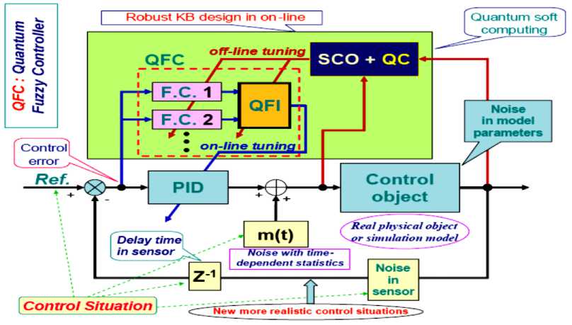


References Thermodynamic trade-off of control performance in quantum fuzzy inference: port-controlled Hamiltonian systems applications
- Haddad W.M., Chellaboina V. and Nersesov S.G. Impulsive and Hybrid Dynamical Systems: Stability, Dissipativity, and Control, Princeton Series in Applied Mathematics, Princeton. - NJ: Princeton University Press, 2006.
- Haddad W. M., Chellaboina V. and Nersesov S. G., Thermodynamics: A Dynamical Systems Approach, Princeton Series in Applied Mathematics Princeton. - NJ: Princeton University Press, 2005.
- A.J. van der Schaft, Theory of port-Hamiltonian systems (Lectures 1, 2, and 3), Network Modeling and Control of Physical Systems. - DISC, 2005.
- Ulyanov S.V. Self-organized control system: US patent № 6, 411, 944, 1997; see also «Self-organization fuzzy chaos intelligent controller for robotic unicycle: A new benchmark in AI control». - Proceedings 5th Intelligent System Symposium. - Tokyo, Sep. 29 -30, 1995. - Pp. 41-46.
- Ulyanov S.V., Panfilov S.A. System and method for stochastic simulation of nonlinear dynamic systems with high degree of freedom for soft computing application: US patent № 0039555 A1, Pub. Date: Feb. 26, 2004.
