Three Dimensional Rapid Brain Tissue Segmentation with Parallel K-Means Clustering Using Graphics Processing Units

The segmentation of medical images is a crucial work due to its unclear boundaries and enormous noise [1]. Magnetic resonance imaging (MRI) is capturing in-depth information of soft tissue organs like brain [2]. Different types of MRI images are T1-weighted, T2-weighted, fluid-attenuated inverse recovery (FLAIR) and proton density (PD). T1-w images are used for analyzing healthy tissues [3]. The primary tissue regions in brain image are grey matter (GM), and white matter (WM) immersed in a fluid called cerebrospinal fluid (CSF) [4]. Segmenting brain tissue from MR images and voluminous is helpful to understand the performance of brain functioning. Several automatic methods are available to segment the brain tissues [5, 6, 7, 8]. Generally, methods are required user inputs and complexity in nature due to the size of MR volume. This gap motivates to propose a fully automatic knowledge based model for brain tissue segmentation with parallel architecture.

K-means is one of the famous clustering algorithms for brain tissue segmentation and its supports parallelism in nature. When using voluminous data, it will be a time-consuming process to cluster the whole data [9]. The parallel implementation of the clustering algorithm overcomes the time-consuming process. Several parallel computing architectures are compute unified device architecture (CUDA), field-programmable gate array (FPGA) and Hadoop. From the literature studies, GPU is well-suited for tasks benefiting from massive parallelism for image oriented problems; FPGAs excel in highly specialized and customizable computations; while Hadoop is geared towards distributed storage. Medical images are massive data so that GPU based parallel architecture is well adopted and customizable in this proposed work.

Graphical processing units (GPU) are used in recent years for performing parallel computations. The primary role of GPU is 3D rendering and high speed in gaming environments that partially utilizes the hardware resources. Thus the modern researchers focus on using the parallel environment while working with extensive data to reduce the computation time. Therefore GPUs are used for medical image operations like image registration, segmentation, classification, denoising etc. from CT, MRI, and PET scanners. The CUDA model works in such a way that the framework supports automatic scheduling of the threads by the GPU hardware [10].

In this decade, rapid growth of medical imaging data expected a high performance computation to produce the high accuracy data on time. Several methods are proposed to accelerate the computation on brain tissue segmentation which assist the doctors to give better treatment on time [11, 12, 13]. Algorithms should adopt the nature of parallel implementation like K-means clustering.

Varity of techniques are available to parallelize the K-means algorithm. Parallel K-means algorithm implemented in CUDA enabled NVIDIA GeForce 8600 with single-dimensional array with one million instances grouped into 4000 clusters [14]. This parallel implementation is compared with a serial K-Means implemented on a 3 GHz Intel Pentium D processor and yielded 13× folds of speed up. Parallel K-Means algorithm is with per-slice threading approach in NVIDIA Quadro K5000 GPU system [15]. They experimented on the speed of the GPU engine by varying the number of slices and concluded that when the number of slices is high, it yields 20× folds of speedup for parallel K-means algorithm.

K-Means clustering algorithm in a multiprocessor environment with the help of shared memory [16]. The initial centres are placed in the shared memory, which is accessible by all the processors. Each processor is assigned n/p instances where n is the maximum number of instances, and p is the number of processors. After all the threads are finished, the tasks got synchronized to calculate new cluster centres. The main purpose of the shared memory system is due to the need for maintaining concurrency over the globally accessible data.

Parallel K-means algorithm can be implemented using MapReduce approach [17]. Here, non-numeric data are preprocessed to get numeric data-parallel. Initialization performs serially followed by parallel membership calculation and cluster assignment. MapReduce is responsible for recalculating the new centres either all centres in a single thread or partial centres for each sub-dataset and finally all are merged in a separate thread. Parallel implementation of K-Means using click plus and OpenMP and CUDA [18]. Images of varying sizes have experimented with a concentration on relatively large data. While parallel implementation, we consider two aspects such as computation and memory. For ccomputation aspect, the proposed method leverages GPU parallelism to accelerate computationally intensive when dataset size increases, the workload can be efficiently distributed across multiple GPU cores, ensuring sustained performance improvements. For memory efficiency, to handle larger datasets, memory-efficient strategies such as batch-wise processing and memory pooling have been implemented to prevent GPU memory overflow. Techniques like data streaming allow for loading and processing data in chunks rather than all at once, significantly reducing memory constraints.

In our current parallel implementation CUDA was selected for the following reasons: CUDA is specifically designed and optimized for NVIDIA GPUs, which are widely used in deep learning and high-performance computing. Its architecture allows for better utilization of hardware resources, leading to improved execution speed and efficiency compared to OpenCL in many cases. In contrast, OpenCL is a cross-platform framework that must work on different hardware architectures (NVIDIA, AMD, Intel, FPGA, etc.), which can lead to suboptimal performance due to the lack of vendor-specific optimizations. CUDA provides an extensive ecosystem with highly optimized libraries such as cuDNN, TensorRT, and Thrust, which significantly accelerate machine learning and image processing tasks. These libraries offer seamless integration with deep learning frameworks like TensorFlow and PyTorch, enhancing productivity. NVIDIA actively supports CUDA with comprehensive documentation, regular updates, and strong community engagement. This makes it easier to implement and troubleshoot GPU-accelerated applications. Many research studies and commercial applications in deep learning and medical imaging leverage CUDA due to its stability and performance. The widespread adoption of CUDA in these domains ensures better reproducibility and compatibility with state-of-the-art methods.

This proposed work aims to segment the brain tissue using parallel K-means implementation in GPU. Histogram based self initialization technique is used to auto initialize the clustering algorithm (HBSKM). Number of clusters (K) and initial centroids (C) automatically calculated from the mid image from the dataset through Gaussian smoothening technique. Working datasets are collected from IBSR repositories which is famous online repositories for testing brain tissue segmentation methods. Then all the image data and inputs were passed to GPU for parallel implementation. Final segmented tissue results were collected from GPU and compared with ground truth results for validation. Under postprocessing, all three tissues are rendered in 3D environment for assessment. The remaining section of the paper are organized in such a way that section, section 2 contains parallel architecture, section 3 the serial and parallel implementation of HBSKM, section 4 contains interpretation and conclusion under section 5.

2.    Parallel Architecture

Several parallel computing architectures are available to handle huge volume of medical data such as GPU, FPGA and Hadoop. From the literature review, all three parallel computing platforms are entirely application and problem dependent. All platforms are having their own merit and demerits. A detailed feature wise comparison is given in Table 1. From the table, we observed that the GPU-CUDA platform is more opt for image processing kind of problems.

• 2.1.    GPU CUDA

  For accelerating computational capability of a system, CUDA is one of the most general parallel programming models introduced by NVIDIA Corporation in 2007. It is an open-source tool with a combination of software and hardware architecture for performing data-parallel computing on GPU without any need for graphics API with extension of C and C++ languages. The structure of the CUDA programming model includes three essential concepts: host, device and kernel. The CPU is considered as host containing primary C language responsible for logical transaction processing and serial computing [19]. It allows developers to harness the computational power of NVIDIA GPUs for various tasks, including image processing.

• 2.1.1.    Workflow of CUDA

Table 1. Comparison of parallel computing platforms feature wise

Feature	GPU	FPGA	Hadoop
Function	Specialized for parallel processing, especially for graphics rendering, AI, and scientific simulations.	Flexible hardware that can be reconfigured for various tasks, including specialized computations, networking, etc.	Software framework designed for distributed storage and processing of large datasets across clusters of computers.
Architecture	Optimized for handling multiple arithmetic operations simultaneously (SIMD architecture).	Configurable hardware architecture with the ability to adapt to specific computational needs.	Software framework built on a distributed file system (HDFS) and MapReduce programming model.
Programming	Typically programmed using CUDA or OpenCL for parallel computing tasks.	Requires hardware description languages (HDLs) like Verilog or VHDL for programming.	Programmed using various languages supported by the Hadoop ecosystem like Java, Python, etc.
Flexibility	Limited flexibility for different tasks but excels at parallel processing for specific applications.	Highly flexible and can be customized for various computational tasks.	Provides flexibility for distributed storage and processing but might not be as customizable as hardware-based solutions.
Power Consumption	Generally higher power consumption due to higher clock speeds and specialized operations.	Can be more power-efficient as they can be configured for specific tasks, reducing unnecessary operations.	Requires a cluster of computers, consuming considerable power, especially in large-scale setups.
Cost	Cost-effective for specific parallel processing tasks but may not be as versatile.	Can be more expensive due to their flexibility and customization options.	Relatively cost-effective for handling large-scale data processing compared to traditional methods, considering hardware and infrastructure costs.
Use Cases	Deep learning, image and video processing, scientific simulations, gaming.	High-frequency trading, IoT applications, aerospace, telecommunications, among others.	Large-scale data analysis, batch processing, and distributed storage in big data applications.

Here is an overview of the CUDA working process for image processing:

Device and Host Memory: CUDA operates on both device (GPU) and host (CPU) memory. Data is transferred between these memories as needed for processing.

Kernel Functions: In CUDA programming, developers write functions called "kernels" that are executed on the GPU. Kernels are designed to perform specific tasks in parallel.

Grids and Blocks: Kernels are executed in parallel by multiple threads organized into a grid of thread blocks. Each thread block contains multiple threads, and threads within a block can cooperate and share data through fast on-chip memory called shared memory.

Image Data Transfer: Images or image data are often loaded into the GPU memory before processing. CUDA provides functions to manage memory transfers between the CPU and GPU.

Parallel Processing: CUDA allows for massively parallel processing of image data. Each thread in a block can be responsible for processing a specific portion of the image.

Optimizations: Developers can optimize CUDA code by carefully managing memory access patterns, utilizing shared memory, and ensuring efficient use of GPU resources to achieve better performance.

Result Retrieval: Once the image processing operations are completed on the GPU, the resulting processed image or data can be transferred back to the CPU memory if necessary.

• 2.1.2.    CUDA GPU Architecture

CUDA Cores and Streaming Multiprocessors (SMs): CUDA cores are the fundamental processing units within an NVIDIA GPU responsible for executing instructions in parallel. These cores are organized into streaming multiprocessors (SMs), each containing multiple CUDA cores, along with shared memory and other specialized units. SMs handle thread execution, manage resources, and perform scheduling of threads.

Memory Hierarchy: CUDA GPUs have different memory types, including global memory, shared memory, constant memory, texture memory, and registers.

Global Memory: Large memory space accessible by all threads. It's relatively slower but has high capacity.

Shared Memory: Fast and low-latency memory that can be shared among threads within the same thread block.

Constant Memory: Optimized for read-only data that is broadcasted to all threads in a block.

Texture Memory: Specialized for optimized access patterns, particularly in graphics applications.

Registers: Each CUDA core has its own set of registers for storing temporary data and variables during computation.

Thread Hierarchy: Threads in CUDA are organized into a hierarchy consisting of grids, blocks, and threads.

Grid: The highest level of organization, containing multiple blocks.

Block: Groups of threads that can communicate and synchronize via shared memory.

Thread: Individual units of execution that run in parallel within a block.

Kernel Execution: Kernels are functions written in CUDA C/C++ that are executed on the GPU. A kernel is launched by specifying the grid and block dimensions along with the kernel function. The CUDA runtime schedules and manages the execution of kernels on the GPU.

Parallelism and Synchronization: CUDA allows for massive parallelism by launching thousands of threads to perform computations concurrently. Threads within a block can synchronize and communicate through shared memory, enabling cooperation and data sharing.

Optimizations and Performance: Optimizing CUDA code involves efficient use of memory, minimizing data transfers between CPU and GPU, utilizing shared memory effectively, and exploiting parallelism for maximum performance.

The CUDA execution and programming model is shown in Fig. 1 and Fig. 2. The implementation of GPU program starts with copying the data from host to device memory. The kernel is launched to perform the data in parallel using the device’s global, shared, local registers, and finally copies back the result from device memory to the host memory [20].

In this proposed work, we used Nvidia GPU (Qudro K5000) which is donated by Nvidia Corporation to support academic research and development. Here are the general specifications of the Quadro K5000 GPU: Architecture: Kepler, CUDA Cores: 1536, Memory: 4 GB GDDR5, Memory Interface: 256-bit, Memory Bandwidth: Up to 173 GB/s, Max Power Consumption: 122W, Bus Type: PCIe 2.0 x16, Form Factor: Dual Slot, Outputs: Display Port (x2), DVI-I DL (Dual Link), a stereo connector, Maximum Threads per Block: 1024, Maximum Block Dimensions: (1024, 1024, 64) and Maximum Grid Dimensions: (2147483647, 65535, 65535).

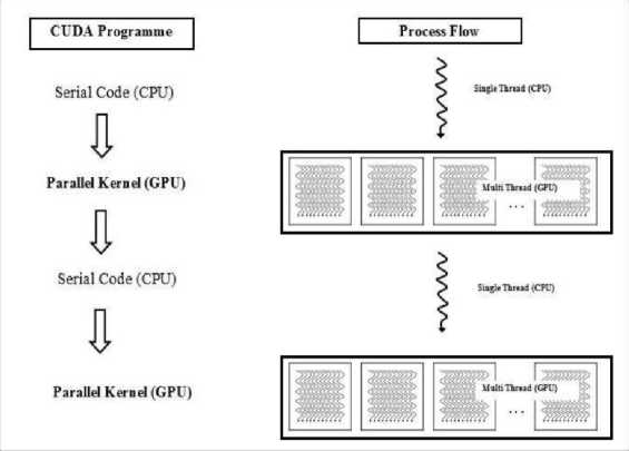
Fig. 1. CUDA execution model

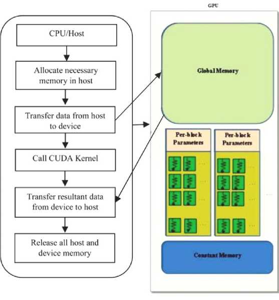
Fig. 2. CUDA programming model

3.    Methodology

The traditional K-means clustering technique involves three stages. The first stage focuses on number of clusters (K) initialization and the initial centres (C). In the second stage, the distance between the data points and centres are computed in order to assign the data point into the minimum distance cluster. Finally, at the third stage, the centres are calculated and replaced as the mean of the clusters. The second and third stages are repeated iteratively until there is no change in the cluster centres. For better understanding, space and time complexity of general K-means algorithms as follows:

Space Complexity:

Input Data: The space complexity for storing the input data is 0 (n * d), where n is the number of data points and d is the number of dimensions (features) in each data point.

Centroids: The space complexity for storing k centroids (each centroid has d dimensions) is 0 ( к * d).

Cluster Assignments: Additional memory may be required to store cluster assignments for each data point, resulting in 0 (n) space complexity for storing cluster labels.

Time Complexity:

Initialization: The initial assignment of centroids is usually 0( к * d) for selecting the initial k centroids.

Assignment Step: In each iteration, each data point is assigned to the nearest centroid. This step has a time complexity of 0 (n * к * d) since for each data point, it calculates the distance to all k centroids in d-dimensional space.

Update Step: After assignments, the centroids are updated by taking the mean of the data points in each cluster. This step involves visiting each data point once to compute the new centroids, resulting in a time complexity of 0 (n * d).

Iterations: The k-means algorithm iterates until convergence, which may take a variable number of iterations depending on the convergence criteria (e.g., minimum change in centroids, maximum number of iterations). The number of iterations can vary, but in the worst case, it can be 0( iter * n * к * d), where iter is the number of iterations required for convergence.

The overall time complexity is usually dominated by the number of iterations, which is highly dependent on the data distribution, initial centroids, and convergence criteria. The development of the proposed work contains three versions of self initialized K-means algorithm. Version I and Version II is homogenous CPU and GPU implementation respectively whereas Version III heterogeneous implementation of both CPU and GPU. Following subsections have explained those implementations.

• 3.1.    Serial CPU HBSKM (Version I)

HBSKM is a fully automatic initialization of the number of clusters (K) and the initial centres (C) for K-means. Initially, algorithm is fully implemented in CPU with serial manner. In this algorithm, the histogram of the middle image in a volume is constructed, and then Gaussian smoothening is performed on the histogram in order to obtain distinct peaks. An image histogram provides a graphical representation of the intensity distribution across the pixels of an image. To determine the number of tissue regions in a brain image, the histogram of the middle slice is analyzed. This slice is chosen because it typically contains all major tissue regions and provides the most frequent intensity values for each region. To enhance the clarity of distinct intensity peaks, a low-pass Gaussian smoothing filter is applied to the histogram, as described in Equation (2). This filtering process helps in identifying distinct peaks that correspond to the different tissue regions present in the brain image. Since the brain primarily consists of three main tissue types— cerebrospinal fluid (CSF), gray matter (GM), and white matter (WM)—the histogram typically exhibits three major peaks. These peaks are used to determine the number of centroids (K) and their corresponding intensity values, where j=1,2,3,...K. The original and smoothed histograms for the middle slice of the IBSR 205_3 dataset, highlighting the distinct peaks, are illustrated in Fig. 3. Fig. 3 does not give any meaning full information like number of clusters (K) and the initial centres (C). From the image, we observed that the more number of pixels are available near zero and that is coming from void background. Under the tissue segmentation, background void region can be avoidable.

Gaussian smoothing filter is mathematically defined as in Eqn. (1).

G ( x ) =

2 πσ

_e 2 σ ²

Where, G(x) is the Gaussian function at position(x), σ (sigma) represents the standard deviation of the Gaussian distribution , x and y are the positions in the filter kernel along the x and y axes.

After applying Gaussian smoothening technique, the same image is shown in Fig. 4. From the smoothened histogram, the number of peaks represents the number of centres (K), and the peak values represent the initial centres (C). In this process, all the inputs automatically taken from the mid image itself without user interaction and it is called knowledge based self initialization. The step by step process of serial HBSKM is given in the Algorithm I [21].

Algorithm I: Serial (CPU) implementation of HBSKM

Step 1: Compute the histogram of the mid image in a dataset.

Step 2: Apply Gaussian filtering on the histogram to get the smoothened the histogram that yields distinct peaks.

Step 3: Find the peak values and their count as C and K, respectively.

Step 4: Applying K-Means segmentation

Step 5: Initialize the final centres of the current slice to next or previous slices

• 3.2.    Parallel GPU HBSKM (Version II)

When we go for large data in clustering into GM, WM and CSF, the proposed HBSKM can be implemented in parallel using GPU threads. The Gaussian smoothened histogram is used for getting initial centroid values from the middle slice of the MRI volume. These centres are fed as input to each thread in the kernel function.

CUDA configuration for parallel implementation as follows: number of thread = number of images X number of volume (20*60), global memory is utilized to process each thread. Number of blocks and grids are automatically calculated from number of threads. Sample CUDA code snippet for thread block and grid computation is given. Synchronization among threads within a block can be achieved using the __syncthreads () function. This function ensures that all threads within a block have reached a certain point in the code before proceeding further.

• #    Example code snippet

block_dim = (256, 1, 1) # Adjust according to the problem size and resource constraints grid_dim = (num_elements // block_dim[0], 1, 1) # num_elements represents the total number of data points if grid_dim[0] * block_dim[0] < num_elements:

grid_dim[0] += 1 # Adjust the grid if the total number of elements isn't perfectly divisible by the block size

• #    Launch kernel with the computed grid and block dimensions

kernel_function<<>>(args)

__syncthreads ()

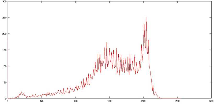
Fig. 3. Histogram of Mid image from 205_3 dataset

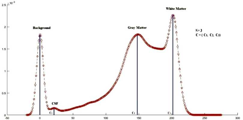
Fig. 4. Histogram smoothing using Gaussian filter

An input array with N * Row * Co I size is created in order to store the entire MRI volume. The Gaussian smoothened histogram is applied to the N/2 th image in order to get k as well as c , , c₂ ... . k_k values. Here k is the number of clusters and c , , c₂ .... c_k are the centres. These values, along with an input array are fed as input parameters to the CUDA kernel. The clus₁, clus₂ .. clus_k are the arrays with N * Row * OoI dimensions where the clustered data are stored in the CUDA kernel. First of all, memory for all the above said variables are allocated and transferred from host memory to device memory. In CUDA kernel, the N numbers of threads are allocated for each 2D slice. The parallel implementation of the K-means clustering is given below.

Algorithm II: Parallel (GPU) implementation of HBSKM

Step 1: Create input, clus₁ , clus₂ …․ clus_k with N ∗ Row ∗ Col dimensions in the host.

Step 2: Read N images as an input.

Step 3: Create C-^ , C^ … and k variables with N ∗ 1 dimension in host memory.

Step 4: Create MS array with Row x Col dimension to store the middle slice.

Step 5: Apply the Gaussian smoothened histogram on MS to get the values for C-y , ^2 …  .

Step 6: Create ^newl ^, Cnew2 …․ ^newk

=    , Сг , C3 .

Step 7: Transfer input, clus₁ , clus₂ …․ clus_k , K, N, C-^ , ^2 …   , ^newl , ^new2 …․ ^newk to device memory.

while (( Ci ^- ^newl || C₂^- ^new2 || C_k ^- ^newk ) == 0.5)

{

Call CUDA kernel for cluster Assignment<<>> (Parameter list)

ci = c = c=

^k =

Call KmeansCentroidUpdate<<>>( clus₁ , clus₂ …․ clus_k , ^newl , ^new2 …․ ^newk ) }

Step 8: Transfer the data from device to memory.

Step 9: Output: The final clus 1 , clus 2 , clus 3 .

Device code (GPU):

Kernel 1: KmeansClusterAssignment (input, clus Y , clus 2 …․clusк, ^1 , ^2 …   )

Id=blockIdx.x * blockDim.x + threadIdx.x;

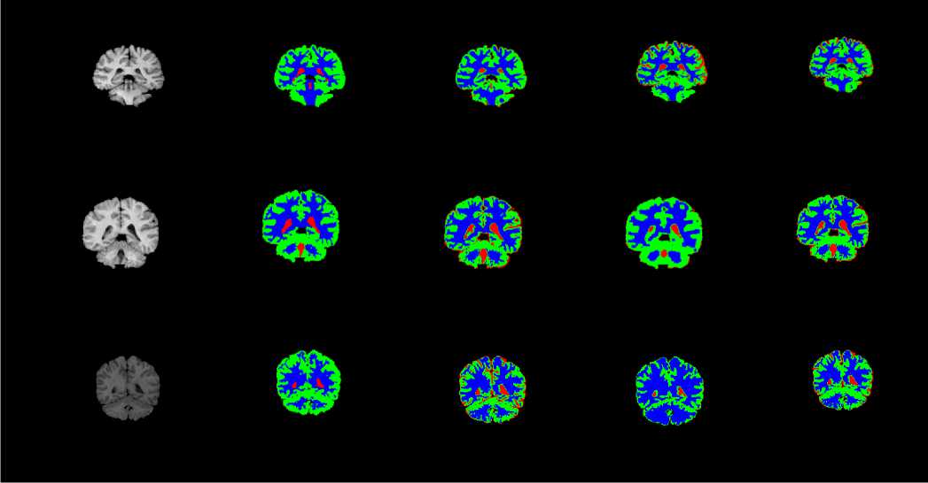
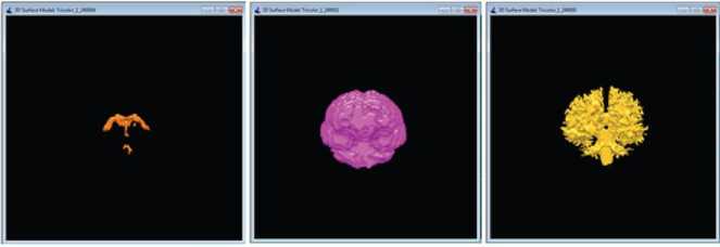
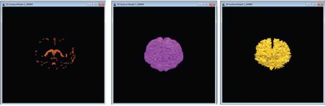
If (Id

Call distance_datapoint_centroid(input(Id), clus1, clus2 …․clusк)

Assign data points to the closest cluster clus1 or clus2or…․or clus к

Kernel II:KmeansCentroidUpdate(input, clus1, clus2 …․clusк, C ,C2 …Ск)

Id=blockIdx.x * blockDim.x + threadIdx.x

If (Id

^newl (Id)=mean (clus₁ (Id))

^new2 (Id)=mean (clus₂ (Id))  .

Qnewk (Id)=mean (clus_k (Id))

• 3.3.    Hybrid CPU - GPU HBSKM (Version III)

Homogenous GPU implementation (Version II) is not impressive because threads are waiting for dependent step like taking summation for centroid calculation. So that heterogeneous parallel implementation is proposed to fuses both CPU and GPU computations for clustering the data points. Version III is very similar like Version except complex cluster assignment of the data points is performed parallel (GPU) whereas summation and centroid calculations is performed in CPU. Step by step process is given in Algorithm III.

Algorithm III: Hybrid (CPU - GPU) implementation of HBSKM

Host code (CPU):

Step 1: Create input, clus , clus2 …․clusк with N∗ Row ∗ Col dimensions in host

Step 2: Read N images into input

Step 3: Create C-y , ^2 … variables with N∗1 dimensions in host memory

Step 4: Create MS array with Row ∗ Col dimension to store the middle slice MS=Input [N/2][1:Row][1:Col]

Step 5: Apply Gaussian smoothened histogram on MS in order to get the value for C-y , ^2 …

Step 6: Create ^newl

new2 ■

'Tiewk

=  , Сг …

Step 7: Transfer input, clus1, clus2, …clusk, K, N, C^ , ^2 …   , ^newl , ^new2 …․ ^newk to device memory while ((Cl - ^newl || C2 - ^new2 ||Ck - ^newk) == 0.5) {

Call CUDA_Kernel :Cluster_Assignment<<< N,1>>>(input, clus^, clus₂ …․clus_k, ^A. , ^2 …  )

c⁼

c u2 =

к=

Call CPU_Function: CentroidUpdate(     ,      …․      ,   ,   …   ,      ,      …․      )

}

Step 8: Transfer the data from device to memory

Step 9: Output are the final      ,       …․

Device code (GPU):

Kernel 1: KmeansClusterAssignment (input, clus , clus …․clus , С ,С …С )

Id=blockIdx.x * blockDim.x + threadIdx.x;

If (Id

Call distance_datapoint_centroid(input(Id),      ,      …․      )

Assign data points to the closest cluster clus or clus or…․or clus

Host code (CPU):

CPU_Function: CentroidUpdate (Parameter list)

{

For i=1:N

{

( )=      (( ))

( )=      (( ))

( )=      (( ))

} return      ,…․

• 4.    Results and Discussion

  The CPU experimental setup was able to Intel(R) Core (TM) i5, Microsoft VS2013 IDE, VC++, and CUDA 8.0 libraries. Experimental datasets are collected from online repository named as Internet Brain Segmentation Repository (IBSR), which contains twenty normal brain volumes with segmented tissues available in the gold standard [22]. The dataset is created by Massachusetts General Hospital. Each volume contains around sixty images with 256 × 256 image resolution and 1×1× 3 mm³ slice thickness. Some of the dataset are affected intensity non-uniformity artefacts given by the MR scanner. Few pre-processing steps included like removal of scalp, skull, eyes, neck, and fat from IBSR20 to improve the accuracy of tissue segmentation [23]. Skull stripping is done by our own developed method called as brain extraction method (BEM2D) [24].

The performance of the HBSKM is measured in terms of Dice score for segmentation accuracy and speedup folds (×) for computation acceleration. Dice coefficient is used to calculate the accuracy of brain tissue segmentation compared with gold standard results. The Dice value ranges between one and zero where one means complete segmentation overlap and zero means no segmentation overlap. Dice score computation is given in Eqn. (2) [25].

Dice Score =

2 x TP

2 x TP+FP+FN

In addition to the Dice segmentation, k-fold validation is taken. K-fold cross-validation is a statistical method used to estimate the performance of machine learning models. The process involves dividing the dataset into K subsets (folds), training the model on K-1 folds, and testing it on the remaining fold. This process is repeated K times, and the final performance is obtained by averaging the results.

Here, given a dataset D with N random samples, divide it into K = 7 sized subsets:

= {   ,   ,․․․,    }

Speedup folds × is considered from the computation time ratio between serial and parallel implementation.

Processing Time in CPU

Speedup folds (x) =------------------------

Processing Time in GPU

The segmented results of the HBSKM and the ground truth results are given in Fig.5. In qualitative analysis, tissue segmentation given by three versions is almost the same. Table 2 shows the qualitative results of tissue segmentation measured using the Dice coefficient. Qualitative results are given in the form of mean ± standard deviation. Therefore, high mean value refers to high tissue segmentation accuracy and minimum deviation stands the stabilization of the method.

The results showed that all three versions gave similar segmentation accuracy. Table 2 showed that the GM, WM and CSF yield 72%, 83% and 17 % of Dice accuracy. In addition to that, k-folds (k=7) cross validation results also included in Table 2 which shows that the model accuracy improved with k-fold validation. The ground truth contains no Sulcal CSF (SCSF). The proposed segmentation results include the SCSF thus got reduced dice score. Ground truth provides SCSF combined with the GM due to their intensity near to GM. Therefore, GM accuracy also got affected. Figure 6 showed the virtual reality of 3D brain tissue segmentation rendered from the output of proposed method and also compared with the ground truth result. This kind of 3D volume helps to estimate the qualitative accuracy of segmentation. 3D visualization helps to the physicians to predict the brain disorders [26]. From the figure 4, proposed method predict the sulcal CSF from the input image but which was ignored in the ground truth CSF computation.

(a)                               (b)                               (c)                               (d)                             (e)

Fig. 5. Qualitative results of proposed versions on brain tissue segmentation (a) Original image (b) gold standard image (c) version I (d) version II (e) version III

(a)

(b)

Fig. 6. Virtual reality of 3D tissue segmentation (a) Ground truth results of CSF, GM, and WM. (b) Proposed segmentation of CSF, GM, and WM

Table 2. Dice Score (mean ± standard deviation) of the HBSKM

Method Name	Dice Score for K=1			Dice Score for K=7
	GM	WM	CSF	GM	WM	CSF
HBSKM Version I	0.71 ± 0.14	0.83± 0.05	0.17 ± 0.10	0.78±0.04	0.83±0.03	0.15 ± 0.10
HBSKM Version II	0.72 ± 0.12	0.82± 0.06	0.15 ± 0.15	0.77±0.08	0.81±0.05	0.14 ± 0.11
HBSKM Version III	0.72 ± 0.14	0.83 ± 0.12	0.17 ± 0.13	0.78±0.02	0.83±0.03	0.14 ± 0.13

Table 3. Comparison of proposed work with several state of an art methods

Method		Brain Tissues
Category	Name	GM	WM	CSF
Existing	KM	0.67 ± 0.14	0.78 ± 0.05	0.13 ± 0.10
	FCM	0.78 ± 0.07	0.74 ±0.04	0.27 ± 0.16
	FFCM	0.69 ± 0.03	0.80 ± 0.04	0.11 ± 0.03
	FAST	0.68 ± 0.06	0.79 ± 0.10	0.13 ± 0.04
	SPM5	0.76 ± 0.06	0.80 ± 0.04	0.17 ± 0.07
	SPM8	0.78 ± 0.06	0.81 ± 0.08	0.21 ± 0.07
	GAMIXTURE	0.77 ± 0.09	0.74 ± 0.02	0.25 ± 0.12
	ANN	0.69 ± 0.09	0.77 ± 0.14	0.15 ± 0.06
	KNN	0.64 ± 0.09	0.80 ± 0.06	0.13 ± 0.04
	FANTASM	0.70 ± 0.10	0.77 ± 0.14	0.15 ± 0.06
	PVC	0.66 ± 0.11	0.63 ± 0.23	0.13 ± 0.05
	FSL FAST	0.77 ± 0.09	0.75 ± 0.05	-
	Hierarchical LS SVM	0.76 ±0.02	0.76 ± 0.04	-
	Hybrid Hierarchical LS SVM	0.78 ± 0.03	0.78 ± 0.03	-
Proposed Methods	HBSKM Version I	0.78±0.04	0.83±0.03	0.15 ± 0.10
	HBSKM Version II	0.77±0.08	0.81±0.05	0.14 ± 0.11
	HBSKM Version III	0.78±0.02	0.83±0.03	0.14 ± 0.13

Table 3 shows that the proposed knowledge based parallel implementation of k means was compared with several state of an art methods. It shows that the proposed methods were competitive result with exiting models. The segmentation results of HBSKM on the IBSR20 dataset are presented in Table. 2 and Table 3. For gray matter (GM), the Dice coefficient ranges from 0.694 to 0.86, with a mean value of 0.78. For white matter (WM), the Dice coefficient varies between 0.66 and 0.91 yielding a mean value of 0.83. For cerebrospinal fluid (CSF), segmentation results range from 0.09 to 0.46 with a mean value of 0.14. The relatively poor performance in CSF segmentation can be attributed to two main factors. First, the intensity values of CSF and GM are very similar in T1-weighted MRI, leading to misclassification. Second, CSF appears as a void black region in T1-weighted MRI, which is sometimes interpreted as background in certain datasets. Table 4 shows that the proposed model evaluated by the various metrics. It shows that the model perform well with the GM and WM segmentation and unable to predict the CSF due to the poor labelling and artefacts.

Table 4. Sensitivity, Specificity, and Accuracy of the

Evaluation Parameters	Tissue Type	HBSKM Version II
Sensitivity	GM	0.7932
	WM	0.9543
	CSF	0.3342
Specificity	GM	0.9846
	WM	0.97309
	CSF	0.9967
Accuracy	GM	0.9660
	WM	0.98357
	CSF	0.99773

Table 5 displays the average computation time per volume taken by the proposed work in all three versions. HBSKM version I is a CPU based serial implementation and takes 43 seconds per dataset. Version II is an entirely GPU based implementation which takes 12 seconds per dataset. This version requires all the data upload into GPU global memory for computation. Huge data transfer between CPU and GPU is a lengthy process. Summation operation inside the GPU is a time expensive process due to the limited speed of GPU co-processors. These two reasons make the full GPU implementation infeasible and provide 3.5× speedup folds than the version I.

Table 5. Average computation time in seconds of proposed works

Method No.	Method Name	Platform	Computation Time (Seconds/Datasets)	Speedup folds (×) CPU VS GPU
1	HBSKM Version I	CPU	43	-
2	HBSKM Version II	GPU	12	3.6x
3	HBSKM Version III	CPU-GPU	07	6 x

Version III is a hybrid method that implements both CPU and GPU. Sequential part utilizes the CPU for execution, and the parallel part runs in GPU. Therefore, during the execution context switch is placed between CPU, and GPU. This process makes the optimum implementation and reduces the computation time up to 7 seconds per dataset. Finally, Version III has given 6× folds speed up than normal CPU execution.

5.    Conclusion

The proposed HBSKM algorithm is applied on the IBSR 20 dataset to cluster the three major tissue regions GM, WM and CSF. K-Means is a hard clustering algorithm popularly known for its simplicity. When the data to be clustered is too large, it leads more time to cluster the data. In such a case, it is feasible to implement in a graphics processing unit. Here three versions of the proposed HBSKM algorithm have been proposed. The version I processes the algorithm serially in the VC++ environment. Version II processes the algorithm parallel and yields 3.5x speedup folds than the serial implementation. Version III is a hybrid version that combines both heterogeneous CPU and GPU implementations yields 6x speedup folds than Version I. Qualitative validation is done through the 3D brain tissue volume estimation.

Acknowledgements

We gratefully acknowledge the support of NVIDIA Corporation Private Ltd., USA with the donation of QUADRO K5000 GPU used for this research. Further, we acknowledge 3D doctor software purchased under the DST project, No: SP/YO/011/2007 used for our results verification. We would like to express our gratitude to the reviewers for their precise and succinct recommendations that improved the presentation of the results obtained.