Threshold controlled binary particle swarm optimization for high dimensional feature selection

Published Online August 2018 in MECS

In many real-world machine learning and data mining problems, classification of datasets into various classes is an important task. This task becomes more challenging when data sets often involve a large number of features. Feature selection is an important process in any classification. It is noted that all the features do not contribute equally as well as significantly in the classification process [1]. Only a few features are relevant for this purpose and rest of the features do not contribute as most of the time they are noisy and redundant. Further, to identify those few important features is a cumbersome task. Also, the large number of features increases the complexity of classifier in terms of time as well as space [2]. So, the process of selecting a compact feature subset from the complicated list of extracted features to reduce the complexity of computation without hampering the accuracy of classification is called feature selection. Hence, one of the most important and challenging problems is to find the minimal set of features which is capable of classifying the dataset with great accuracy. In this way, feature selection becomes the most crucial task in the process of classification. If we consider all features for analysis, the problem will become very complex which leads to a large search space and consequently making it NP-hard problem [3]. Therefore, a process known as feature selection is required. Feature selection is a process which aims to reduce complexity in real-world data by choosing a subset of relevant or necessary features from a reservoir of redundant, irrelevant and unnecessary attributes of the data. This selection process may increase the accuracy of the analysis model and reduces dimension.

Feature selection approaches are mainly divided into two categories on the basis of their evaluation pattern: Filter approach and Wrapper approach. In filter approach [4], features are being scored by using some statistical information measures, such as information gain, mutual information gain, chi-square, TF-IDF, etc., without using any classifier and predictive model. Here, features are selected on the basis of correlation with their outcome variables obtained from various statistical tests. In wrapper approach [1], feature subset selection depends on the classification algorithm. Here, features are wrapped around the classifier used. Forward and backward feature selection, recursive feature elimination are the popular example of wrapper methods. In general, filter methods are faster and less expensive but poor in results as compared to wrapper methods. The wrapper-based approach is considered to develop the model and the scope of this paper.

Due to large search space, traditional exhaustive search techniques are unable to solve the problem of feature selection. In general, there are total 2 ” possible solutions exist for a dataset with n features, which grows exponentially with the value of n. Due to this limitation, Evolutionary Computation (EC) based techniques have gained a lot of attention and used to a greater extent among the research community in recent years. EC is a collection of many population-based approaches which are derived from the nature-based evolutionary system. These approaches are used worldwide in most of the engineering and scientific optimization problems.

In the domain of feature selection, these EC based approaches have been utilized in very limited manner, and among them, Particle Swarm Optimization (PSO) [5, 6] has been used to some extent. The underlying reason behind the less utilization of these approaches is that the number of features considered is very large varying from thousand to hundreds of thousands. Therefore, suffers from convergence problems due to very high dimension. PSO, proposed by Kennedy and Eberhart [5], is one of the most explored and extensively used EC based approaches because of its algorithmic simplicity and computational efficiency [7]. Although, PSO is widely used in feature subset selection problems, yet it still has many limitations. The primary limitation is that sometimes PSO is trapped into local optima due to multimodality nature of the problem. Another, limitation is that the performance of PSO decreases as the number of features increase because of the curse of dimensionality. Both the variants of PSO, continuous and binary, have been utilized for high-dimensional feature selection and classification in many types of research [8, 9]. Researchers have tried to improve the performance of PSO algorithm by making changes into various stages like representation scheme of particles, initialization strategies of particles, calculation of fitness function and search mechanism of particles.

Since feature selection is discrete in nature, therefore Binary PSO (BPSO) is the most feasible method to fulfill the requirement. Most of the research performed in this area considered the binary variant of the evolutionary algorithm. The sigmoidal function is used to map the continuous variant of the evolutionary algorithm into binary. BPSO also uses the sigmoidal function to convert the continuous PSO (CPSO) into BPSO. Therefore, the performance of BPSO is highly depended on the functioning of sigmoidal function which is used to convert the continuous values of particle’s velocities into discrete values as per formula is given below.

0  if Г and()-S( v(t+1))

(c + 1)   {1 if rand()

where S (·) is the sigmoidal function for mapping the values of the velocity over [0.0, 1.0] as per the following expression:

S И ; ■ Mi _ •.. .

and r a nd() is the pseudo-random number uniformly distributed over [0.0, 1.0].

This formula clearly indicates that selection of a feature for the next iteration solely depends on the randomly generated value by rand() function. For example, a feature having the high value of ( ( + 1))

as 0.83 may be discarded for the next iteration if generated random value is greater than 0.83 but a feature having a low value of S(v( t + 1)) as 0.03 may be selected for next iteration if generated random value is less than 0.03. Secondly, if generated random value is very small like 0.001 than features having values of S(v( t + 1)) as 0.003 and 0.73 or 0.93 will have equal chance to be selected for next iteration. So, more often this random value leads to the selection of unfit features and rejection of potential features. In this case, the convergence of BPSO algorithm will be get delayed and chances of getting optimal solution decrease.

This phenomenon was also highlighted by Tran et al. [10] in their research. They described that a feature is selected if its probability is greater than a predefined threshold. Therefore, two evolved probabilities, one is slightly greater than the threshold and the other is significantly greater than the threshold, have the same effect on the solution, which may limit the performance of BPSO for feature selection. They, again, in their work [11] reflect that less than 5% of a total number of features in all the datasets are responsible for classification accuracy. Rests of the features are redundant and noisy and need to be discarded by feature selection algorithm. Hence motivation was received for our proposed research work.

In this research, a new threshold instead of using () is proposed in the formula of position update in BPSO. New proposed approach selects the minimum number of features for high-dimensional datasets and classifies the datasets with great accuracy. This research makes the following contributions:

• 1.    New threshold controlled BPSO (TCBPSO) which always is capable to select a minimum number of features with high accuracy.

• 2.    TCBPSO is never got trapped into local optima irrespective of a high number of features in all the datasets.

• 3.    TCBPSO reduces the number of features selected in all the high dimensional datasets.

• 4.    Multi-Class Support Vector Machine (MC-SVM) is used to classify the data on selected features.

The performance of the proposed approach will be evaluated by experimenting on small and large datasets. The rest of the paper is organized as follows. Related work is discussed in Section II, Section III presents the problem formulation, the concept of PSO and BPSO is discussed in Section IV. Section V presents the concept of SVM, experimental results are thoroughly discussed in Section VI and Section VII ends the paper with the conclusion.

• II.    Related Work

Feature selection from high-dimensional data using PSO has been studied by many researchers. Various papers are being published with different techniques to improve the selection of important features.

Alba et al. [12] propose two hybrid techniques PSO/SVM and GA/SVM where PSO and GA are augmented with support vector machine respectively. These techniques are employed on high-dimensional DNA microarray data for the selection of informative genes.

Fong et al. [13] propose a Swarm search to find optimal features. They utilized many swarm-based algorithms like PSO, BAT, and WSA for selection of optimal feature set over some high dimensional data set. But, their high-dimensionality is only limited up to 875 only.

Tran et al. [14] aim to develop a new PSO approach PSO-LSRG which combines a new local search on pbest and a reset gbest mechanism for feature selection in highdimensional data sets.

Dara et al. [15] proposes binary PSO with Hamming distance and is employed on the high-dimensional gene data. The hamming distance, a similarity measurement technique, is used here for faster convergence of the solution as well as for reduction of irrelevant features. This approach has not reduced the size of optimal feature set sufficiently.

Doreswamy et al. [16] combine the clustering techniques and stochastic techniques to obtain the effective features. The fast K-means, a variant of K-means is embedded for feature selection from high dimensional data.

Fahrudin et al. [17] exhibit the power of ant colony algorithm in high-dimensional and noisy data over the evolutionary algorithms GA and PSO.

Shenkai et al. [18] aim to use a variant of swarm optimization known as competitive swam optimization (CSO) to select relevant features from a larger set of features. The experimental results show that the CSO outperforms the traditional PCA-based method and other existing algorithms.

The paper [19] aims to present improved shuffled frog leaping algorithm (SFLA) to predict the relevant features in the high-dimensional biomedical dataset. On comparison with popular algorithms of feature selection, SFLA gives better results in terms of identification of important features. But, the accuracy achieved for almost all dataset is very low.

Tran et al.[20] propose a new hybrid PSO-based approach (PSO-LSSU) where the evolutionary process of PSO combines wrapper method and filter method. PSO-LSSU obtains higher accuracy classification and lesser time for the feature selection of higher dimensional data. However, for some datasets, average test accuracy is still very low and complexity of the algorithm is very high.

Typically, the feature selection techniques are applicable to the discrete data. The discretization loses the impact of the interaction of features. Keeping this in mind, the authors [10] combine the process of discretization and feature selection technique to improve the feature selection. They proposed particle swarm optimization (EPSO) method and FS in a single stage using barebones particle swarm optimization (BBPSO). Classification accuracy of various datasets is not satisfactory and optimal numbers of features selected are quite high.

They further proposed a new method called potential particle swarm optimization (PPSO) to reduce search space and improve the results [11].

• III.    Problemformulation

The objective of this data classification problem is to maximize the classification accuracy at the cost of minimum selected features. To obtain the desired level of accuracy a multi-objective fitness model is developed which contains Accuracy, Selected Features and Total Features of the problem and is associated with a weight factor. The fitness function is given in (3).

SF

Min. fitness = α ∗ (  ) + (1 - α) ∗ (1 - Accuracy)

(3) where

α = Weight parameters

SF = Number of Selected Features TF = Number of Total Features Accuracy =Classification Accuracy

The weight parameters (α) will be chosen according to the need. In this case, α is taken as 0.15 because we want a high level of accuracy that’s why 85% weights are provided to the second term. A number of features selected through BPSO will be SF and when these selected features will be passed to SVM then the classification accuracy will be considered as Accuracy.

• IV.    Particle Swarm Optimization

• A.    Particle Swarm Optimization

  PSO was first proposed by Kennedy and Eberhart in 1995 for solving continuous optimization problems known as Canonical PSO. Since then a large number of variants of PSO have been proposed and applied successfully to several continuous and discrete optimization problems. This nature-inspired algorithm is induced by the behavior of birds and got inspired by its collective, collaborative and self-learning behavior. Here, each bird or swarm is termed as a particle which is a source of better performance for another swarm. PSO is a population-based metaheuristic algorithm which is approximate and non-deterministic in nature. It works by maintaining a population of swarm or particles. Each particle depicts a candidate solution which consists of two components of the particle in a given search space. They are position and velocity. In each iteration, position and velocity of every particle are updated not only on the basis of its own personal experience but also on neighboring particles experience. The best position achieved so far by an individual particle is depicted as pbest and the best position of particle among all the particles in the group is denoted as gbest. On the basis of these pbest and gbest, PSO searches for the optimal solutions in the search space by updating the velocity and the position of each particle according to the following equations:

Vid1 =   ∗ Vfd + Cl ∗ rl∗(Pid - ^id)+C2 ∗ r2

∗(Pad - -^id )(4)

^d1 =   +Vid1(5)

/                x maxiter-iter ,,

W=( ^mtn ^- ^max )∗         ₊ ^max (6)

Here, t denotes the t ^th iteration in the search process and d ∈ D represents the d ^th dimension of the particle in the search space. w is called as inertia weight, which is to regulate the impact of the particle’s previous velocities on the particle’s current velocity. c₁ and c₂ are termed as acceleration constants. r1 and r2 are random numbers which are uniformly distributed & generated in [ 0, 1]. p id is the pbest of i ^th particle in the d ^th dimension and p gd is the global best particle gbest at the t ^thiteration in the d ^th dimension. The velocity is clamped by a predefined maximum velocity, v max , and v ∈ [-v max , v max ]. There is two main stopping criterion of the algorithm. One is when algorithm reaches the predefined maximum number of iterations and second, the algorithm achieves a desired fitness value.

• B.    Binary Particle Swarm Optimization

Kennedy and Eberhart introduced the BPSO algorithm which allows the PSO algorithm to operate in binary problem spaces. It uses the concept of velocity as a probability that a bit (position) takes on one or zero. In the BPSO velocity is updated which remains unchanged, but for updating the position is re-defined by the rule given in (1) and (2). The pseudo code of BPSO is shown in Algorithm 1. It should be noted that the BPSO is susceptible to sigmoid function saturation, which occurs when velocity values are either too large or too small. In such cases, the probability of a change in bit value approaches zero, thereby limits exploration. For a velocity of 0, the sigmoid function returns a probability of 0.5, implying that there is a 50% chance for the bit to flip. However, velocity clamping will delay the occurrence of the sigmoid function saturation. Hence, optimal selection of velocity is important for faster convergence.

Algorithm 1: Feature Selection based on Binary Particle Swarm Optimization (BPSO)

• 1:    Initialize parameters of BPSO

• 2:    Randomly initialize particles

• 3:    WHILE stopping criterion not met DO

• 4:     calculate each particle's fitness value

• 5:    For i = 1 to populationsizeDO

• 6:        update the gbest

• 7:         update the pbest of i^th particle

• 8:    END

• 9:   FOR i = 1 to population sizeDO

• 10:      FOR j = 1 to dimension of particleDO

• 11:                  update the velocity ofi^thparticleaccording to

equation (4)

• 12:           update the position ofi^thparticleaccording to equation

• 13:     END

• 14:    END

• 15:    END

• V.    Support Vector Machine

Support vector machine (SVM) is machine learning classifier based on supervised learning which is used for various classification tasks. SVM is a computationally good learning approach proposed by Vapnik et al. [21,22]which finds optimal separating hyperplane through learning. The goal of SVM is to design a hyperplane that classifies all training vectors into various classes. If the number of classes is only two then SVM is known as linear SVM otherwise it is known as non-linear SVM. The best choice of the hyperplane is which leaves the maximum margin from all the classes. The margin is the distance between hyperplane and the closest elements from this hyperplane. The equation of hyperplane can be given as

a∗х+b=0            (7)

where a is a weight vector and b is a bias (scalar). The maximal margin is denoted mathematically by the formula as in (8) where ||w|| is the Euclidean norm of w.

m = _|| w||

The goal is to minimize the w or maximize the total margin which leads to non-linear optimization task and solved by the Karush-Kuhn-Tucker conditions using Langrage multipliers a n and given as:

f(х т)=∑n=l ynanхT+b0         (9)

where хT is a test instance yn is the class label of support vector хn an is a Lagrangian Multiplier bQ is a numeric parameter n is the number of support vectors

• VI.    Results and Discussion

In this paper Threshold Controlled Binary Particle Swarm Optimization (TC-BPSO) based feature selection method is proposed and compared with Conventional Binary Particle Swarm Optimization (C-BPSO) to evaluate the performance of proposed approach. In C-BPSO the rand() decides whether the feature will select or not while in TC-BPSO a predefined threshold decides the selection of a feature. The threshold varies from 0.5 to 0.9 in order to check the impact of varying threshold on efficiency. Ten machine learning datasets are taken from standard repositories [23, 24] to test the performance of the proposed algorithms as given in Table 1. The datasets taken are different in nature, some having a very small number of features, some have a large number of features, and some have just two classes while some of the datasets having many classes. These combinations of datasets are taken to check whether the proposed approach perform effectively in all context or not. Classification accuracy of these datasets is calculated using Multi-Class SVM (MC-SVM). MC-SVM model is used to calculate the classification accuracy of the datasets having either two or more than two class.

Table 1. Datasets

S.No.	Datasets	Total Features	Total Instances/ Samples	Total Classes
1	DLBCL	5469	77	2
2	Prostate Cancer	10509	102	2
3	9 Tumors	5726	60	9
4	11 Tumors	12533	174	11
5	SRBCT	2308	83	4
6	WBCD	32	569	2
7	Breast Cancer	9	699	2
8	Parkinson’s	22	195	2
9	Lung Cancer	56	32	3
10	Wine	13	178	3

Datasets are split into training and testing sets. 70% of the data used for the training while rest 30% of the data used for testing. Classification accuracy is calculated on test data. Datasets having various range of instances i.e. minimum 32 to maximum 699 are taken to check the training efficiencies of MC-SVM model. On the other hand, minimum 10 to maximum 12533 features are taken to check the performance of proposed C-BPSO and TC-BPSO algorithms. PSO parameters taken in both the cases are shown in Table 2.

Table 2. C-BPSO and TC-BPSO parameters

Parameter Name	Value
Inertia Factor	^min =0.95 ^max =0.99
Acceleration Constants	Cl =   = 2.05
Velocity	=-6         =6
Number of particles	10
Maximum iteration	100

A. Feature selection results on small datasets

Datasets numbered from 6-10 in Table 1 is considered as small datasets because it contains a small number of features. While the datasets numbered from 1-5 are considered as large datasets due to its large features. Experimental results on these datasets using C-BPSO are presented in Table 3. Results using TC-BPSO are shown in Table 4. Since the feature selection methods, C-BPSO and TC-BPSO are stochastic in nature. Hence, the results of these datasets are calculated by performing 30 independent runs, then their best, average, and worst results are listed. In each run, both the feature selection algorithms iterated up to maximum iteration. Best accuracy is marked bold in Table 3 and Table 4.

Table 3. Experimental results of C-BPSO

Datasets	Measures	Accuracy (in %)	Features Selected
	Full	100	5469
DLBCL	Best	100	2346
	Average	100	2359.6
	Worst	100	2371
	Full	96.77	10509
Prostate	Best	100	4771
Cancer	Average	99.46	4729.36
	Worst	96.77	4680
	Full	27.78	5726
9 Tumors	Best	44.44	2535
	Average	43.51	2593.87
	Worst	27.78	2786
	Full	75	12533
11 Tumors	Best	76.92	5711
	Average	75.77	5996.5
	Worst	75	6169
	Full	100	2308
SRBCT	Best	100	857
	Average	100	880.37
	Worst	100	901
	Full	98.25	32
WBCD	Best	99.42	7
	Average	99.03	10.92
	Worst	98.25	14

	Full	99.04	9
Breast	Best	100	5
Cancer	Average	99.28	4
	Worst	98.57	3
	Full	74.14	22
Parkinson’s	Best Average	86.21 82.76	9 10.43
	Worst	79.31	9
	Full	30	56
Lung	Best	100	13
Cancer	Average	94.33	18.13
	Worst	90	10
	Full	100	13
Wine	Best Average	100 99.37	6 5.83
	Worst	98.11	7

Table 4. Experimental results of TC-BPSO

#D	#M	Accuracy in % (Features Selected)
		0.5	0.6	0.7	0.8	0.9
#1	#F	100 (5469)	100 (5469)	100 (5469)	100 (5469)	100 (5469)
	#B	100 (2579)	100 (119)	100 (11)	100 (4)	100 (5)
	#A	100 (2607)	100 (140.3)	100 (12.33)	100 (5)	100 (7)
	#W	100 (2626)	100 (168)	100 (15)	100 (7)	100 (8)
#2	#F	96.77 (#PC)	96.77 (#PC)	96.77 (#PC)	96.77 (#PC)	96.77 (#PC)
	#B	100 (5117)	100 (251)	100 (30)	100 (21)	100 (10)
	#A	99.03 (5154)	99.11 (255.6)	100 (54.5)	100 (35)	100 (12.7)
	#W	96.77 (5098)	96.77 (220)	100 (93)	100 (56)	96.77 (7)
#3	#F	27.78 (5726)	27.78 (5726)	27.78 (5726)	27.78 (5726)	27.78 (5726)
	#B	38.89 (2786)	55.56 (168)	72.22 (37)	77.78 (28)	77.78 (28)
	#A	37.50 (2782)	53.34 (180.5)	65.28 (58.5)	71.43 (33.29)	70.63 (31.3)
	#W	33.33 (2734)	50.00 (192)	55.56 (108)	66.67 (47)	61.11 (35)
#4	#F	75 (#11T)	75 (#11T)	75 (#11T)	75 (#11T)	75 (#11T)
	#B	75 (6075)	80.77 (331)	86.54 (93)	86.54 (76)	90.39 (91)
	#A	75 (6142)	79.80 (377.7)	84.14 (111.3)	85.00 (70.8)	85.58 (83.7)
	#W	75 (6229)	76.92 (408)	80.77 (76)	82.69 (69)	82.69 (100)
#5	#F	100 (2308)	100 (2308)	100 (2308)	100 (2308)	100 (2308)
	#B	100	100	100	100	100

		(1073)	(58)	(31)	(10)	(15)
	#A	100 (1085)	100 (65.75)	100 (37.25)	100 (24.75)	100 (17)
	#W	100 (1095)	100 (72)	100 (53)	100 (32)	100 (21)
#6	#F	98.25 (32)	98.25 (32)	98.25 (32)	98.25 (32)	98.25 (32)
	#B	98.83 (14)	98.83 (6)	99.42 (11)	99.42 (7)	98.25 (5)
	#A	98.25 (13)	98.25 (8.25)	98.54 (8.5)	98.83 (7)	97.90 (5.8)
	#W	97.66 (11)	97.66 (9)	97.66 (7)	98.25 (6)	97.66 (7)
#7	#F	99.04 (9)	99.04 (9)	99.04 (9)	99.04 (9)	99.04 (9)
	#B	99.52 (4)	99.52 (4)	99.04 (3)	99.52 (4)	98.57 (2)
	#A	99.23 (3.6)	99.40 (3.75)	98.65 (2.5)	98.81 (2.6)	98.41 (2)
	#W	99.04 (3)	99.04 (3)	98.09 (2)	98.09 (2)	98.09 (2)
#8	#F	74.14 (22)	74.14 (22)	74.14 (22)	74.14 (22)	74.14 (22)
	#B	82.76 (3)	82.76 (2)	82.76 (1)	86.21 (5)	82.76 (1)
	#A	82.07 (7.4)	82.41 (4)	82.76 (3.4)	83.45 (2)	82.47 (1.33)
	#W	81.03 (11)	81.03 (4)	82.76 (8)	82.76 (2)	81.03 (1)
#9	#F	30 (56)	30 (56)	30 (56)	30 (56)	30 (56)
	#B	70 (22)	90 (9)	80 (7)	90 (10)	70 (2)
	#A	65 (24.33)	77.5 (8.75)	80 (8.83)	80 (7.2)	66.67 (4)
	#W	60 (33)	70 (9)	80 (10)	70 (4)	60 (4)
#1 0	#F	100 (13)	100 (13)	100 (13)	100 (13)	100 (13)
	#B	100 (5)	100 (5)	100 (5)	100 (5)	100 (5)
	#A	99.05 (6.5)	99.05 (5.25)	99.24 (4.8)	99.53 (5.5)	97.40 (4.13)
	#W	98.11 (8)	98.11 (5)	98.11 (4)	98.11 (5)	96.22 (4)
#D- Datasets #M- Measures #5- SRBCT #8- Parkinson’s #F- Full #W- Worst		# 1- DLBCL # 3- 9 Tumors # 6- WBCD # 9- Lung Cancer # B- Best #PC-10509		# 2- Prostate Cancer # 4- 11 Tumors # 7- Breast Cancer # 10- Wine # A- Average #11T- 12533
In the above tables, the classification accuracy at selected features is compared with the classification accuracy at original features. The accuracy of both the feature selection algorithm is evaluated by considering

the same fitness function as explained in problem formulation section.

• 1.    C-BPSO versus Full Features

• 2.    TC-BPSO versus Full Features

  In TC-BPSO the classification accuracy is also significantly better than the accuracy at full features like C-BPSO. The feature reduction, in this case, is also better than the C-BPSO. The maximum reduction in features is observed for “Prostate Cancer” dataset. TC-BPSO method reduces total features in “Prostate Cancer” dataset by 99.99904%. While the maximum improvement in accuracy is observed for “Lung Cancer” dataset. In “Lung Cancer” dataset the accuracy improved by 60%.Thus both the methods achieved the goal by replacing redundant and repeated features in order to increase the classification accuracy.

• 3.    TC-BPSO versus C-BPSO

It is clearly seen in Table 3 that the classification accuracy in all cases is significantly better than the accuracy at full features. Moreover, the C-BPSO method not only improves the accuracy but also drastically reduces the features. The maximum reduction in features is observed for “WBCD” datasets. C-BPSO method reduces total features in “WBCD” datasets by 78.12%. While the maximum improvement in accuracy is observed for “Lung Cancer” dataset. In “Lung Cancer” dataset the accuracy improved by 70%.

As discussed above that a predefined threshold is used in TC-BPSO while rand() as a threshold is used in C-BPSO. Experimental results of C-BPSO is presented in Table 3 while Table 4 contains the experimental results of TC-BPSO. Experiments are conducted by varying the threshold from 0.5 to 0.9. During the experiments, it is observed that a predefined threshold limit the exploration capability. At some threshold, C-BPSO outperforms TC-BPSO while at some threshold C-BPSO underperforms TC-BPSO.

• a.    TC-BPSO at 0.5 threshold (TC-BPSO ^0.5 ) vs C-BPSO

Premature nature of convergence found in TC-BPSO when the threshold is 0.5. Changes are observed only for few iteration, no matter how many iterations are given. As discussed in section 4 that the 0.5 probability occurs when velocity becomes 0 i.e. the bit has 50% chances to get flip. When all the particles achieve zero velocity then the system is said to be converged and then no changes can be observed. Therefore, due to early convergence, the TC-BPSO0.5 underperforms C-BPSO in almost all cases. But as we increase the threshold the classification accuracy increases with strict feature selection mechanism.

• b.    TC-BPSO at rest of the thresholds vs C-BPSO

As the threshold increases from 0.6 to 0.9, the feature selection mechanism becomes stricter. From experiment, we found some important correlation.

• (i)    Almost in all cases which has a large number of features, TC-BPSO outperforms C-BPSO.

• (ii)    In some cases which has a fewer number of features, TC-BPSO underperforms C-BPSO.

• (iii)    TC-BPSO is averagely 3-4 times computationally faster than C-BPSO in all cases.

• (i)    As seen in Table 4 that the classification accuracy in “Prostate Cancer” and in “11 Tumors” are more when the threshold is 0.9. As discussed in Section I that only 5% of the features are responsible for global optima. Therefore, in these two cases, even the strictest selection criteria outperform all due to the availability of large features. Since the total features available in these two cases are 10509 and 12533 and 5% of these features (525 and 626) will be responsible for global optima. Hence, TC-BPSO^0.9 came out with the best accuracy in 100 iterations. The reason for 0.9 threshold to compete in 100 iterations in large datasets is their selection criteria in the 1st iteration. In the 1st iteration, it only selects 10% of the features which is the most favorable condition to converge in 100 iterations. While TC-BPSO at different threshold could also find the best accuracy if the number of iteration is more. At rest of the datasets, TC-BPSO^0.9 underperforms some other variants of TC-BPSO even though the best accuracy is same in some cases like in “DLBCL”, “9 Tumors”, “SRBCT”, and in “Wine” datasets. When the two variants of TC-BPSO returns the same accuracy then the best variant is selected by comparing their average accuracy. If both the best and average accuracy is same then a number of features decide the best variant. On both the large datasets TC-BPSO^0.9 outperforms C-BPSO in all contexts. On “Prostate Cancer” dataset total features get reduced by 54.6% in C-BPSO while total features reduction in TC-BPSO^0.9 is 99.999%, which is 45.40% more than C-BPSO. C-BPSO reduces 54.43% features on “11 Tumors” datasets while TC-BPSO^0.9   reduces

99.993% features, which is 45.56% more than C-BPSO. Comparison of classification accuracy at full features and at selected features using C-BPSO and TC-BPSO approaches are shown in Fig 1.

Computational Efficiency:

Computational comparison on these two datasets between TC-BPSO0.9 and C-BPSO is presented in Fig 2.As seen in Fig 2 that average running time on “Prostate Cancer” in both the cases (C-BPSO and TC-BPSO) is much less than the “11 Tumors”. Average running time on “11 Tumors” is more because it tops the list in terms of number of features, it has more instances than “Prostate Cancer”, and most importantly it has a maximum number of classes.

Through experiment, it is observed that as the number of classes/categories increases, computational complexity significantly increases. However, as computational complexity increases the performance of C-BPSO drastically degrades. Therefore, in “11 Tumors” dataset, the average running time of C-BPSO is 5.6232 times more than TC-BPSO while it is just 1.6680 times more on prostate cancer dataset.

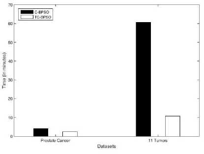
Fig.2. Average running of C-BPSO and TC-BPSO on two large datasets

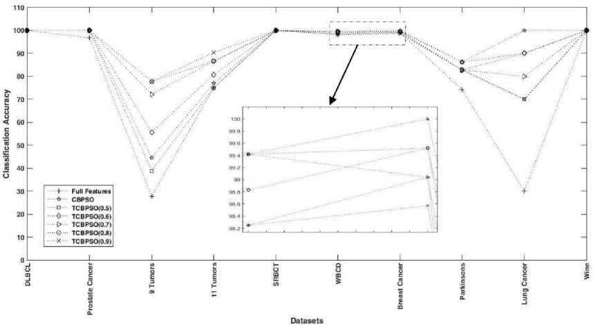
Fig.1. Comparison of classification accuracy at full features and at selected features using C-BPSO and TC-BPSO

• (ii)    In the previous case, we observed that TC-BPSO^0.9 performed well only on two large datasets while TC-BPSO^0.8 performed considerably well on all datasets. Although, through experiment, we observed that if we increase the number of iterations then the best accuracy can be achieved through TC-BPSO^0.8. Even, the accuracy can be achieved if we perform multi-run like 100, 200 etc. though the probability is minimum at some datasets. Such as, the probability of getting best accuracy in “Prostate Cancer” dataset is high while it is low at “11 Tumors” dataset. Hence, all goals such as features reduction, accuracy maximization, and computational complexity minimization can be achieved by setting the 0.8 threshold.

• 4. Comparison with existing methods:

In some cases all the variants of TC-BPSO underperform C-BPSO. As we consider the case of “Breast Cancer” and “Lung Cancer” datasets, the accuracy in C-BPSO is slightly higher than the TC-BPSO. On “Breast Cancer” dataset the classification accuracy in C-BPSO is 100% while it is 99.52 in TC-BPSO0.6, which is only 0.48% less than C-BPSO. However, total features selected in both the cases are 5 and 4. If we consider the case of “Lung Cancer” then the best classification accuracy in both the cases i.e. in C-BPSO and TC-BPSO are 100% and 90%, which is just 10% higher than TC-BPSO0.8 while the selected features at these accuracies are 13 and 10.The reason for less accurate classification accuracy in TC-BPSO is due to their strict selection mechanism because on small datasets selection and rejection of a single feature can either significantly improve or severely degrade the classification accuracy. Like large datasets where many combinations return global optima, the number of combinations which gives global optima is very less on small datasets and flipping of a single bit can impact the accuracy. As for example in “Lung Cancer” case, we observed that when number of features selected were 6 the classification accuracy was 60% when 7 it was 70% when 8 it was 80% and it was 90% when selected features were 9. Therefore, addition and removal of a single feature can either increase or decrease the classification accuracy by 10%. Both the datasets (“Breast Cancer” and “Lung Cancer”) in which C-BPSO outperforms TC-BPSO top the list in containing a minimum number of features.

Best results obtained in proposed work are compared with the best results of some existing work as shown in Table 5. As seen in Table 5 that the proposed approach selects the minimum number of features as compared to the methods proposed by authors [20, 25]. TC-BPSO not only selects the minimum number of features but also improves the classification accuracy.

Results are compared on eight datasets and TC-BPSO outperforms on seven datasets both in terms of features and accuracy. Maximum difference of 17.78% in accuracy is observed for “9 Tumors” while the maximum difference of 2660.3 in features selection can be seen for “Prostate Cancer” dataset. Conversely, the proposed approach underperforms for “11 Tumors” datasets with merely 0.33% difference in terms of accuracy. Additionally, the proposed approach is 5-8 times faster than the approach suggested by authors [20, 25].

Table 5.Comparison results of existing work with the proposed work

Datasets	Features Selected	Best Accuracy (in %)	Approach Used
SRBCT	59.7	100	PSO-LSSU [19]
	10	100	TC-BPSO0.8
DLBCL	1417	93.72	PSO-LS [19]
	4	100	TC-BPSO0.8
9 Tumors	2551.6 46.7	60 60	PSO [19] PSO-LSSU [19]
	28	77.78	TC-BPSO0.8
Prostate Cancer	2670.3	91.17	PSO-LSSU [19]
	10	100	TC-BPSO0.9
11 Tumors	266.8	90.72	PSO-LSSU [19]
	91	90.39	TC-BPSO0.9
Wine	6	100	PSORWS [24]
	5	100	TC-BPSO0.8
WBCD	6	94.74	PSORWS [24]
	7	99.42	TC-BPSO0.8
Lung	5	90	PSORWS [24]
	10 13	90 100	TC-BPSO0.8 C-BPSO

• VII. Conclusion and Future Work

In this paper, a new PSO based dimensional reduction approach (TC-BPSO) is proposed and is compared with Conventional PSO (C-BPSO) approach as well as some existing approach. The goal of this paper is to remove the redundant and repetitive features in order to reduce the dimension as well as to increase the classification accuracy. Therefore, the fitness function used in this paper considers number of features selected as well as classification accuracy. The Same fitness function is used in both the cases to achieve the goal. Multi-Class Support Vector Machine (MC-SVM) based supervised machine learning model is used to calculate the classification accuracy.

Experiments are performed on 10 different datasets having varying difficulties to evaluate the performance of the proposed approach. The results obtained through experiments on these datasets indicate that the proposed approach outperforms in all context such as feature selection, accuracy, and computational complexity. Features selected through the proposed approach are much less than the C-BPSO as well as the existing approaches. Although, the accuracy is also significantly better than these approaches. TC-BPSO is averagely 3-4 times computationally faster than C-BPSO while it is averagely 5-8 times faster than the existing methods. As discussed in results and discussion section that the fixed threshold limits the exploration capability. Hence, a local search strategy will be incorporated in the future in order to remove the exploration capability limitation problem so that the method can also perform well on small datasets.