Time Series Forecasting Model Based on Discrete Grey LS-SVM

Published Online January 2015 in MECS

• I.    Introduction

  Time series prediction refers to the process by which the future values of a system is forecasted based on the information obtained from the past and current data points[1]. At present, there are a lot of methods for time series prediction, from traditional statistical method such as Auto Regressive Moving Average model to artificial intelligence based approaches. Grey system theory is an interdisciplinary scientific area that was first introduced in early 1980s by Deng[2]. Since then, the theory has become quite popular with its ability to deal with the systems that have partially unknown parameters. A grey prediction model is one of the most important parts in grey system theory, and that, the GM(1,1) model is the core of grey prediction[3].Because the grey prediction model needs little origin data, has simple calculate process and higher forecasting accuracy, it has been widely used in the time series prediction of a lot of research fields.

The GM(1,1) model is widely discussed and studied in the grey system[2,3]. The purpose of GM (1, 1) model is to work on system forecasting with poor, incomplete or uncertain messages. The GM (1,1) is based on the grey generating function, which uses the variation within the system to find the relations between sequential data and then establish the prediction mode. However, many scholars find that there are many theory defects in traditional GM (1,1) model[4], and do a lot of researches for this[5,6,7,8]. Discrete GM(1,1) (DGM(1,1))model is a new grey prediction model, which improve some problem existent in original GM(1,1)[7]. However, the parameters estimation method of the DGM(1,1) is still by means of least square method. Least square method is based on empirical risk minimization (ERM) principal, which is large sample principle[9]. Furthermore, the GM(1,1) forecasting study is small sample prediction, estimating parameters based on least square method does not match with the small sample modeling concept. On the other hand, the robustness of the least square method is poor, which affects the stability of the DGM(1,1) model[6,10]. To sum up the above reasons, it is not suitable to estimate DGM(1,1) model parameters by means of least square method.

According to the above describing, we need find a new method to improve the precision of DGM(1,1) model. Recently, a new intelligent approach support vector machine (SVM) has gained popularity due to its many attractive, analytic and computational features, and promising empirical performance[9,11,12]. It is a promising technique owing to its successful application in classification and regression tasks[13,14]. SVM comprises an important class of learning algorithms based on statistical learning. Moreover, SVM is established based on the structural risk minimization(SRM) principle. It shows the good generalization ability. Least squares support vector machine (LS-SVM) has received considerable attention for the last few years due to its simplicity in problem formulation and implementation. It was first proposed by Suykens and Vandewalle[13]. LS-SVM is a least square version for SVM that involves equality instead of inequality constraints and works with a least squares cost function, which leads to the advantages of fast convergence, high accuracy and low computational efforts[11,13]. LS-SVM has been successfully applied to real application modeling considered as a non-linear function regression problem.

For a time series prediction problem, the core of these models is to establish a prediction model[2]. However, in the actual forecast, the same problem can have many different forecasting methods. Given many approximation methods, it has become difficult for an engineer to select the most appropriate method for the problems under study[15]. So it would be very meaningful if different methods can be combined, which consolidates the advantage of the different models and obtains better forecasting accuracy. Based on the approach of “mixture of experts”, some researchers have integrated the GM(1,1) and the artificial neural network to enhance the prediction according to their complementary merits[16,17]. The moving average autoregressive exogenous prediction model is combined with grey predictors for time series prediction[18], and it is proved that the hybrid method has a greater forecasting accuracy than the GM(1,1) method. Another study introduces a support vector regression grey model (SVRGM) which combines support vector regression (SVR) learning algorithm and grey system theory to obtain a better approach to time series prediction[19].

Both the grey model and the SVM model do not need to know whether the prediction variables obey normal distribution, do not to require too much statistic sample. However, each has some defects. The primary interest of this paper lies in combining the two models: DGM(1,1) forecasting model and LS-SVM forecasting model. Based on the theoretical analysis, a new idea or algorithm is put forward. This paper establishes a new DGM(1,1) time series prediction model based on LS-SVM algorithm, which is a combination of DG (1,1) and LS-SVM with their respective advantages, grey theory is used to conduct accumulative sequence of the raw data, and the least squares support vector machine is adopted for the SRM and prediction.

The remainder of this paper is organized as follows: Sec.2 are brief overviews of DGM(1,1) and LS-SVM. Then a time series prediction model based on discrete grey least squares support vector machine is established in Section 3. Experimental results are given in Section 4. Finally, conclusion is drawn in Section 5.

• II.    Review on DGM(1,1) model and LS-SVM

• A.    DGM(1,1) model

Definition! Let X ⁽⁰⁾ = ( x ⁽⁰⁾ (1), x ⁽⁰⁾ (2), - ■ ■ , x ⁽⁰⁾ ( n )) is a sequence, where x ⁽⁰⁾ ( k ) >  0, k = 1,2, • • •, n and X⁽¹⁾ is the accumulated generating operation (1-AGO) sequence of X ⁽⁰⁾, X ⁽¹⁾ = ( x ⁽¹⁾ (1), x ⁽¹⁾ (2), - ■ ■ , x ⁽¹⁾ ( n )) ,

Where

k x (1)( k) = ^ x (0)( j),( k = 1,2, ■■■, n) j=1

x ⁽¹⁾( k + 1) = в x ⁽¹⁾( k ) + в                    (1)

Then (1) is called a DGM(1,1) model, or the discrete form of a GM(1,1) model[7].

T

Theoreml: If в = ( в , в ) is a sequence parameters and

x(1) (1)1

x(1) (2)1

x (1)( n —1)1

x ⁽¹⁾(2) x ⁽¹⁾(3)

x ⁽¹⁾ ( n )

Then the least square estimate sequence of the grey differential (1) satisfies в = (BTB )—1 BTY.

Theorem2: If B , Y and в are stated in theorem1, then let x (1)(1) = x (0)(1), k = 1,2,--*, n-1, then x (1)( k +1) = #x (0><1) + 1-4 p2                (3)

¹ P 1

The restored values, k = 1,2, • • •, n — 1, then

x ⁽⁰⁾ ( k + 1) = x ⁽¹⁾ ( k + 1) — x ⁽¹⁾ ( k )                   (4)

The traditional DGM(1,1) model has the following problem:

(1)The DGM(1,1) estimates parameters based on least square method, which does not match with the small sample modeling of GM(1,1).

(2)The robustness of the least square method is poor, which affects the stability of the model.

• B.    LS-SVM algorithm

Giving a training set {(xk, yk)}"=1, xk e Rn, yk e R, where x is the k -th input sample, y is the desired output value . LS-SVM has been developed for solving an approximation problem. It allows the construction of an approximation by mapping the initial data set implicitly into some high dimensional feature space Z through some mapping ^(x) . LS-SVM aims at constructing an simple linear approximation in the feature space Z then corresponds to a nonlinear approximation in sample space[20].

All can be done implicitly in Z by means of the kernel function K ( x , x _y) = ф ( x ) ^T ф ( x _y) . LS-SVM models take the form:

f ⁽ x ) = w^T p ⁽ x ) + b                              ⁽⁵⁾

where w e R ^k is weight vector and b e R is bias term. To obtain w and b one solves the following constrained optimization problem[13]:

N min- llwll + — У ^2

w , b Л 2^{11  11}      2^_x (6)

s.t.  yk = wT9(xk) + b + ^k, k = 1,2," N where ^k is a error variable, X > 0 is tradeoff parameter between a smoother solution and training errors.

To solve the optimization problem, the Lagrange function can be defined as follows:

N

L (w, b, ^a) = - ||w|| + -£ ^k k=1

N

^- Z ^a k [ w T Ф ( x k ) + b + 5 k ^- У к ]

k = 1

where a_k are Lagrange multipliers. The solution of α and b is given by

e

e

T

b

α

y

N x N

where, e = ( 1,1,---1 1 , T

1x N and Q = (к (x, Xj )) nx n .

Finally, we substitute w into Eq. (1) and thus the training sets of nonlinear approximation is obtained too,

N f (x) = Za kK( Xk, x) + b                    (9)

k = 1

The selection of the kernel function has several possibilities. It is arbitrary symmetric function, which meets the Mercer theorem[9], such as:

• (1)    linear Kernel: K ( x ., x _y) = X T Xj

• (2)    polynomial Kernel of degree d:

K ( x , x₃ ) = ( x T Xj + c ) , c >  0

Where c is a parameter.

• (3)    Kernels generating Gaussian radial basis function(RBF):

K ( x , X j ) = exp{-

x- x j 172^2}

Although grey forecast and LS-SVM forecast build on the basis of different theories, there are some similarities between DGM(1, 1) and LS-SVM. Both of their study is small sample prediction. DGM(1,1) by identifying the parameters of the model is actually based on the least squares linear regression, whereas support vector machine is evolved from the linear optimal surface. Both models have their own advantages and weaknesses. DGM(1,1) is a model of the difference equation, which strengthens the regularity of raw data by cumulative generation; moreover, it is the fitting of exponential curve. However, the DGM(1,1) estimates parameters by means of least square method[7], it requires too much statistic sample to ensure the ability of the model, and it need to require the prediction variables obey normal distribution, despite the grey model itself does not make demands on data distribution. On the other hand, the robustness of the least square method is poor, which affects the stability of the model. LS-SVM is a theory based on SRM, which has very good generalization ability[19]. LS-SVM method does not need to require the prediction variables obey normal distribution.

Based on the above analysis, combining the two above mentioned small sample prediction methods, a new grey LS-SVM model named DGM(1,1) LS-SVM is proposed to overcome these limitations on both of the two forecasting models. The fluctuation of data sequences is weakens by the grey theory, and the generalization ability of the model is enhanced by the statistical learning theory, and the DGM(1,1) LS-SVM is a combination of those advantages.

Above all, the DGM(1,1) is used to conduct a cumulative sequences of the raw data, and is employed to choose the kernel of the LS-SVM, on the other hand, the LS-SVM algorithm is adopted for the process and prediction.

Theorem3: If ф₂, Pi) T is the grey differential (1) parameters and

For this equation, a is a positive real constant which can be adjusted by users. Because Gaussian RBF kernels tend to give good performance under general smoothness assumptions, since Gaussian RBF function is usually used as a kernel function. The precision and convergence of LS-SVM are both affected by X and a . The selection of parameters of a SVM model is important to the accuracy of the forecasting. Most SVM practitioners select these parameters empirically by trying a finite number of values and keeping those that provide the least testing error[21].

Unfortunately, now there is no unified method to select the parameters of the model.

e   ф( x ^^г>^)ф( x ^(1>) ^T + —

where e = ( 1,1,---1 ) ^T    _n, X >  0 ,

1 x ( n - 1)

I =

, Y =

,

¹   -    1 ) ( n - 2) x ( n - 2)

L У J

III. Discrete Grey Least Squares Support Vector Machine

Against defects in a single model described above, a new discrete GM(1,1) time series prediction model based on LS-SVM algorithm is established.

y = LX(1) (2), X(1) (3), ■ • •, x(1) (n) JT, and_ ф(x(1)) = (x(1) (1), x(1) (2), • • •, x(1) (n -1))T. Then the

LS-SVM algorithm estimate sequence of the grey difference (1) satisfies

Г₽2 1

(BTB)"' BTY

7 2 x n

Proof: To consider

x ⁽¹⁾( k + 1) = 0 1 x ⁽¹⁾( k ) + 0 2 , k = 1,2,-, n - 1,    (10)

taking {(x(1)(k),x(1)(k +1))}n 1 as a training set, k=1

coefficients ( 0 , в ) T can be obtained as solution to the following optimization problem based on LS-SVM algorithm,

^ n x 1

= ( B ^T B ) ^{- 1} B T Y , according to

ф ( x ⁽¹⁾) = ( x ⁽¹⁾ (1), x ⁽¹⁾ (2), -, x ⁽¹⁾ ( n - 1)) ^T ,

min - || в II² + — У 0 2

Pi,Р2Л 211/1112 ^

s.t.  x (1)( k +1) = px (1)( k) + в + 0, k = 1,2,---n -1

To solve the optimization problem, one defines the Lagrange function

L ( 0 , 0 2 , 0 , a ) = ¹ К + ^A £ 0

^{2         2} k = 1                      (12)

- £ « k [ 0 x ⁽¹⁾( k ) + 0 2 + 0 - x ⁽¹⁾( k + 1)] k = 1

0i = £ akx (1)( k) = ф( x(1))T a k=1

hence f 02 )J 1    0  )f

( 0 J ( 0   ф ( x ⁽¹⁾) ^T \   ( a J ,

17                        /2xn7n

= f 1     °. J  (BTB)-1 BTY(15)

I 0    ф ( x ⁽¹⁾) ^T J₂

X             7

DGM(1,1) model can be expressed

5c(1) (k +1) = £ a,.x(1) (i)x(1) (k) + 0(16)

i = 1

where a = [a_T, a₂, • • •, a^ ] T are Lagrange multipliers. By Karush-kuhn-Tucker conditions, the conditions for optimality are[13]

' d L 5 0 1	= 0	^	« = £ - : a . v-i k ), k = 1
S L_ 5 0 2	= 0	^	£ > ; a = 0, k = 1
d L 5 ^ t	= 0	^	a k = A^ k
d L ®ak	= 0	^	0 x (1) ( k ) + 0 + 0 - x (1)( k + 1) = 0

where k = 1,2, • • •, n - 1 .

After elimination of 0 and 0 , the solution is given by

e

e ^T

^ф( x ⁽¹⁾⁾ф⁽ x ^(1>) T + i

к

n X n

α

y

f 1  -  1"

^{where e} = (^1,1,-"¹) 1 x ( n - 1) T , I =  ■         :

l ¹  -  Ц n - 1) X ( n - 1)

^a = [ ^a_Pa 2 ,-, a n - 1 ] T , y = [ x ⁽¹⁾(2), x ⁽¹⁾(3),-, x ⁽¹⁾( n ) ] T ф ( x ⁽¹⁾) = ( x ⁽¹⁾ (1), x ⁽¹⁾ (2), • • •, x ⁽¹⁾ ( n - 1)) ^T .

e

Let B =

e

ф ( x '1’M x -¹' ) ^T + 1

A

, Y =

y

, then

Let K(x(1)(i), x(1)(k)) = x(1)(i)x(1)(k) , where the function K is linear Kernel Kernel function. Formula (16) can be expressed n-1

xc ⁽¹⁾( k + 1) = _£ a, K ( x ⁽¹⁾( z ), x ⁽¹⁾( k )) + 0          (17)

i = 1

(17) is a LS-SVM model based on DGM(1,1), we call it a DGM(1,1) LS-SVM model.

Let x(1)(1) = x(0)(1), then restored values, xc(0) (k +1) = 5c(1) (k +1) - 5c(1) (k) = £ ax(1) (i)x<0) (k) i=1

k = 1,2,---, n - 1 .                                 (18)

Based on linear Kernel function, we can get a new method:  DGM(1,1) based on LS-SVM(LS-SVM

DGM(1,1)). The LS-SVM training procedure involves a section of the kernel parameter and the tradeoff parameter. From (17), we can see that we only use linear Kernel to represent the Kernel function of DGM(1,1) LS-SVM. There is only one parameter A need to be made certain, and the number of parameters of this LS-SVM is smaller than other kind of SVM. On the other hand, the AGO functions can transfer the disordering series into monotone raising ones, which provided LS-SVM learning with reasonable data base, the uncertain factors are decreased. For DGM(1,1) modeling based on LS-SVM, the fluctuation of data sequence is weakened by the grey theory and the support vector machine is adopted for the SRM, so the LS-SVM DGM(1,1) machine is a combination of those advantages[5].

In fact, formula (18) gives the DGM(1,1) LS-SVM model expression for fitting. We now discuss the forecasting problem of a DGM(1,1) LS-SVM model.

(1) If k = n , then

i = 1

( n - 1              A                          (19)

V i = 1                 )

(2)Ifk = n +1,n + 2,---, because x(0)(k) is unknown, therefore x(1) (n) is also unknown, now based on iteration forecasting value can be described as follow:

i = 1

i = 1

Combining (19)and (20) ,one arrives at n -1

<                    i = 1                                              (21)

the later development trend of raw series X ⁽⁰⁾ can be forecasted.

• IV. Calculation Example Analyses

In order to test the accuracies of the models in this paper, we now use the following example to carry on the experiment. The raw series [8]demonstrate as follows:

The first six data are taken as the original training samples, the latter 3 data as test samples. The results obtained by the models in this paper are compared with traditional GM(1,1) model and DGM(1,1) model.

Various models are formed in this paper:

> GM(1,1): GM(1,1) model.

• > DGM(1,1): Discrete GM(1,1) model.

> LDGM(1,1): DGM(1,1) LS-SVM.

The results of the identification can be described as Figure 1-3.The “ ﹡ ” expresses the actual value, the real line is the model value. Figure 1 is the identification which uses the GM(1,1) model. Figure 2 is the identification which uses the DGM(1,1) model. Figure 3 is the identification, which uses the DGM (1,1) LS-SVM model.

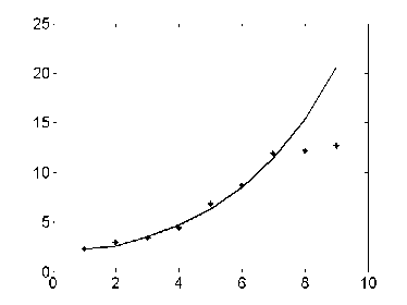
Fig. 1. The identification based on GM(1,1)

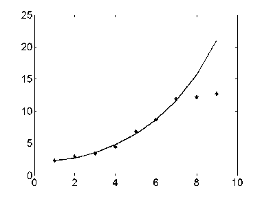
Fig. 2. The identification based on DGM(1,1)

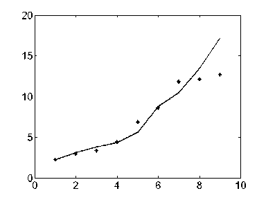
Fig. 3. The identification based on LDGM(1,1)

To demonstrate the accuracy of above models, the actual value and the predicted value can be compared. Eqs.(22)-(24) are the three accuracy evaluation standards that are used to examine the accuracy of the models in this study.

• 1)    The average absolute error:

1l l i=1

• 2)    The average absolute relative percentage error:

  l

  MARPE = -₂

  ^l i = 1

  
  
  

• 3)    The mean square relative error:

  MSRE =

  
  
  

where y is the actual value, and y ˆ is the predicted value.

The result of the identification can be described as` Table 1-2. Table1 shows the identification index on training samples of different methods.

Table 1. Index on training samples of different methods being compared

Index	GM(1,1)	DGM(1,1)	LDGM(1,1)
MAE	0.2366	0.2208	0.3345
MARPE(%)	5.2684	5.1859	6.4692
MSRE(%)	6.6529	6.5368	9.1104

Table2 shows the identification index on test samples of different methods

Table 2. Index on test samples of different methods being compared

Index	GM(1,1)	DGM(1,1)	LDGM(1,1)
MAE	1.9292	2.0150	1.1956
MARPE(%)	15.411	16.085	9.613
MSRE(%)	27.769	29.395	15.873

Figure1-3, show that the training samples are approximate to exponential distribution. Table 1 show that the fitting effect of GM(1,1) and DGM(1,1) model is good. That is to say, the precision, with applying the GM(1,1) and DGM(1,1) model to forecast an approximate exponential incremental sequence is satisfactory. However, it can also be noticed in Figure1-3, in test samples, nonlinear feature is strong, for comparison, the forecasting performance of GM(1,1) and DGM(1,1) model is inferior to LDGM(1,1). The result of the identification is listed in Table 2.

Based on LS-SVM algorithm, LDGM(1,1) find a balance between a smoother solution and training errors, thus the forecasting accuracy of this model in this paper is higher than that of a single GM (1, 1) model or the DGM (1,1). Figure3 shows that the generalization performance of LDGM(1,1) is improved. LDGM(1,1) is capable of processing nonlinear adaptable information. Table 2 shows that the better generalization performance and forecasting accuracy are achieved in LDGM(1,1).The results demonstrate that the prediction accuracy of new model are superior to a single model, which exhibits excellent learning ability with fewer training data and the generalization capability.

In summary, it can be concluded that LDGM(1,1) model shows excellent learning ability with fewer training data, and combines the advantages of DGM(1, 1) and LS-SVM.

• V. Conclusion

A new discrete grey least squares support vector machine is proposed in this paper as a method for time series prediction. This algorithm combines the advantages of DGM(1, 1) and LS-SVM. Through an example’s program simulation, the validity and practicality of this model is verified. Although the proposed model overcomes the defects of parameters estimation in traditional DGM(1,1) model, they may be superior to other modeling methods in some aspects. There are some potential drawbacks such as the selection of tradeoff parameter related to a least squares cost function. The performance of this model is more related to the selection of trade-off parameter. Thus, how to quickly and accurately select the model trade-off parameter should be further studied.

Acknowledgment

This paper is supported by the Hubei province Nature Science Fund of China(2013CFA053) and Open Research Fund Program of Institute of Applied Mathematics Yangtze University of China(KF1506).