Time Synchronization under 1PPS Signal in Distributed Real-time Simulation System

Published Online December 2010 in MECS

• I.    I NTRODUCTION

  Satellite navigation is widely used in many application fields since GPS system came forth in the early 1970s. By now, many similar systems like GLONASS in Russia, GALILEO in Europe are developed. Simulation of these satellite navigation systems, especially of the radio navigation signal in laboratory is valuable in many engineering research fields, such as aviation and vehicle. In order to produce the radio signal, several special physical equipments are evolved in the simulation, so the simulation is a kind of hardware in the loop simulation (HILS). Since there are usually several isolated components, including computers and equipments, in the system, distributed structure is adopted. Above all, production of the radio signal with high precision is a strict real-time task, and so the system is identified as a distributed real-time simulation system.

One of the key points of the distributed real-time simulation system is the time synchronization. This paper studies a time synchronization method based on the simulation system of satellite navigation signal. System structure is illustrated briefly at first. And then, the time synchronization structure is put forward in detail, at the same time, 1PPS signals, and synthetic disturbances in the procedure are analyzed. Thirdly, several synchronization methods are studied under the structure. Since the physical experiment to study the time synchronization method under 1PPS signal is not easy to do. A method of simulation with Arena software is put forth in this paper, which is much more convenient in practice. At the end, some experiments are carried out to prove the efficiency of the time synchronization method.

• II.    HILS SYSTEM STRUCTURE

A Components of the System

Fig.1 illustrates the system structure of the HILS simulation system of satellite navigation signal. It is composed of four parts: a simulation manager, a real-time model subsystem, a signal production subsystem and a time server.

Simulation manager is the interface computer with the whole system, where the man operates, controls and monitors the simulation procedure.

Real-time model subsystem is one of the key components of the simulation system. For a high precise radio frequency navigation signal production, the arithmetic simulation models are complex and the calculation of them is time consuming. Satellite constellation, navigation data coding and pseudo range

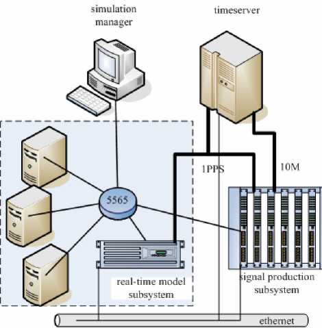
Figure1 HILS system structure calculation would exceed the ability of one single computer, so more than one computer must be gathered together to do the calculation concurrently. All these calculations must be done in real-time, so we call these computers simulating arithmetic models "real-time model subsystem". The subsystem is a distributed system by itself, composed of industry computers from Advantech Corporation.

Signal production subsystem is another key component of the simulation system. Since the physical radio frequency signal production is acquired, the processing such as base band processing, code modulation, D/A and up-converting and so on, must be done, some specific equipments are indispensable. High precision is required, for example, the precision of carrier wave of the navigation radio signal to produce is within 5 millimeters. So, the processing to produce the navigation radio signal is much more critical in time than those arithmetic model calculations in “real-time model subsystem”. In fact, it is usually called rigorous real-time system compared with ordinary real-time simulation system, such as HILS of industry pipelining. Commercial industry computers can’t satisfied with the critical time requirements and the tremendous data processing of the radio signal production, specific boards built with DSP and FPGA are needed. VXI bus is chosen to integrate these boards and we named it as “signal production subsystem” in our system.

Time server is the absolute time source of the system. It is composed of precise atomic clock synchronized with UTC and acts as the server for time synchronization. Multiple time signals are sent out from the server as the standard clock. At the same time, time server provides SNTP services as well. All the multiple time signals and SNTP services must be coherent all the time.

B Connections of theComponents

Besides these four components, there are three kinds of “network” to connect the distributed components. One is the signal coaxial cable, (identified as thick dark line in Fig1.), which is used to transfer the physical time signals to the distributed equipments. The detail of time signals will be described in the next section.

Another network is GE Reflective Memory (RM), which is a typical real-time network in the distributed system. The newest and highest performance RM product offered by VMIC(GE) is the 5565 series. This series operates at 2.1 gigabaud and transport data up to 174 M byte/s. RM network consists of three parts: node cards, hub and multimode fiber. There are two kinds of node card, VMIPCI5565 for PCI industry computers in realtime model subsystem and VMIPMC5565 for VXI computer in signal production subsystem. Since RM is a fiber-optic daisy-chain ring, it’s not convenient to connect fiber. VMIACC 5595 is the managed hub designed to operate with the VMIC’s VMIxxx-5565 family of RM real-time network products. The RM hub can automatically bypass ports when it detects a loss of signal or the loss of valid synchronization patterns, allowing the other nodes in the network to remain operational. RM network serves an important role in realtime communication in the distributed simulation system.

The third network is the normal Ethernet network, which is used to connect all the distributed computers, providing a convenient communication method for those data not so time critical as those sent by RM network.

So the whole system is a distributed hardware in the loop simulation system, and time synchronization must be carried out among these components and equipments.

Ш TIME SYNCHRONIZATION

A Time Synchronization with 1PPS

From Fig.1, we know that time server must provide time source for both real-time model subsystem and signal processing subsystem. Signal processing subsystem is time critical, because it produces the physical radio frequency signal. Signal processing needs to use the external standard clock instead of its own crystal oscillator, so time server must transfer physical sin wave signal of 10MHZ. The sine wave signal is converted to some other signals of different frequency as needed. Except for the sine wave signal, 1PPS signal is also sent from time server as the reference point of time. Both sine wave signal and 1PPS come from the same single crystal oscillator and are transferred by coaxial cable (Thick dark line in Fig.1). The signal processing subsystem is composed of DSP and FPGA cards, and processes the input clock signals by hardware chips, which is not the purpose of this paper.

We concentrate the other part of the system, such as real-time model subsystem, composed of common computers. Time synchronization carried out by computer is much more widely used. Although many time synchronization methods based on Ethernet communication are studied abroad, the synchronization accuracy is approximate milliseconds in the LAN system, which can not satisfied the requirement of navigation signal simulation. What is more, in order to improve the synchronization accuracy, much more packets are to be transported through the Ethernet, which decreases the performance of the network. And the simulation computers have to do some extra programming work to cooperate, which would depress some of its calculation ability of simulation models. Introduction of 1PPS, on the contrary, would eliminate these disadvantages and get much more accuracy, less communication packets and less load of simulation computer.

1PPS signals play an important role in time synchronization, so, an extra PCI card needs to be taken to process the 1PPS signal. When a 1PPS signal arrives, the time card must trigger a PCI interrupt, and an interrupt service routine (ISR) is called to run. Since most work of time synchronization logic is done in host by the ISR, capturing the 1PPS and trigger a PCI interrupt is enough for the time card. So we have a lot of choices to select the card and choose the PCI-1780 from Advantech Corporation in our system.

To synchronize with the time server, the first thing is to capture the pulse signal and initialize with the coming 1PPS signals. One of the most important things is to check the correctness of the signals, which means the signal pulses are sent exactly one per second. If the time intervals are not stable, we can't capture the signal and can't accomplish the time initialization, and an error message must be reported.

So the intervals between the 1PPS signals must be measured in order to check the correctness. The measure may be done by the local crystal oscillator, which may contain error by itself. That is a dilemma, how can we distinguish the error between the input signal and the local timer? An admissible error ε is chosen to cope with the problem. If the error from the intervals of the input pulses exceeds ε measured by local timer, the 1PPS signals are assumed to have error and time synchronization can't be done. If the error, on the other hand, is less than ε, the 1PPS signals are confirmed. The error between the 1PPS signal and the local timer is assumed to belong to local timer, and then the error is used to adjust the local timer.

Another point in the capture is that the 1PPS signals must be stable and contain no noise pulses. If a false pulse signal is checked during the capture procedure, it is assumed to be a valid one. Since the interval between the valid 1PPS signal and a false one is of error larger than ε, it is assumed that the 1PPS signals are not stable and will stop the procedure. Several seconds later, capture procedure is resumed again.

From the description of synchronization logic, we know that an interrupt is assigned to the PCI1780 card on the computer, and it is triggered on each coming pulse. So, the interrupt latency is added to the time delay of the 1PPS signal, it is crucial to the time synchronization. Different interrupt latencies exist in various operating systems. In order to have better accuracy, a professional real-time operating system, Vxworks, is adopted, which is widely used in real-time application field. So the capture procedure is carried out under Vxworks, and the interrupt delay of the ISR is about 2 microseconds [1]. This precision is much better than in ordinary windowsXP operating system. The ISR supported by Vxworks is designed to process the interrupt as below:

• a)    For the first interrupt triggered by pulse signal, record the local time as variable "t1" and then return;

• b)    For the second interrupt, record the time as variable "t2", and return;

• c)    For the third interrupt, record the time as "t3", and check if the logic expression "(|t2-t1-1|<ε)&&( |t3-t2-1|<ε)" is TRUE. Capture procedure is completed on TRUE, and the time frequency error of local crystal oscillator is assumed as "(t3-t1)/2". Rewind and repeat the operation from a) on the condition of FALSE.

From our measurements, the error of the local crystal oscillator is less than 0.7 milliseconds per second, and the interrupt latency of Vxworks is less than 2 microseconds, so we set two milliseconds to the value ε in our project.

B Time Synchronization with SNTP

To do time synchronization in distributed system, 1PPS signal is helpful but not enough; since the simulation time not the physical time is to be synchronized. Software has to be engaged in this task. So, time server must provide "soft" time service except for the physical signal. In our system, SNTP (Simple Network Time Protocol) is adopted by time server, and so Ethernet connection is applied in the system.

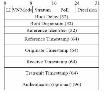
• Figure 2 SNTP time packet

SNTP is a simplified copy of NTP (Network Time Protocol), which is widely used to provide the mechanisms to synchronize time and coordinate time distribution in a large, diverse internet. Rfc documents [2, 3] give a detailed description of NTP and SNTP, so this paper just put forward the structure of the net packet in Fig.2. This packet is adopted to help synchronization between the time server and real-time target subsystem through Ethernet by TCP/IP protocol. Time server works under server mode, while the real-time target node sends request to it as a client. The schedule of synchronization is left to the client to simplify the realization of the time server. Since the 1PPS signals is coherent with NTP service on the time server, the client simply sends an Ethernet request to the time server on receiving a 1PPS signal. The returning time packet from the time server contains the current simulation time. Only the integer of seconds in time packet is used to tag the 1PPS signal, and the fraction is discarded. Because the latency of the SNTP service is usually within a few milliseconds, the integer of seconds in the time packet can precisely tagged the 1PPS signal. Tagging the 1PPS signal is done only once at the initialization period of simulation experiment. The time maintenance is left to the client through 1PPS signal, and SNTP service needs not to be used anymore, unless another simulation experiment starts.

C Time Maintenance with 1PPS Signals.

Once the 1PPS signal is captured and tagged with simulation time at the beginning, simulation time must be kept synchronized all along with the 1PPS signals.

Another task of the maintenance procedure is to create a sub step timer. Since the real-time operation done by the real-time model subsystem is on the step much less than one second, as the interrupt by 1PPS signals. In our project, the sub step is 20 milliseconds.

Two methods can be adopted to set the sub step timer, first is the watch dog timer from Vxworks and the other is the counter interrupt from PCI1780.

Watch dog timer is more convenient than the latter. A " wdFunc()" procedure is created first, user codes handling the 1PPS interruption are put into the procedure, and a system function " wdCreate() " is used to create watch dog timer, and the timer is triggered by system function " wdStart ()". There are some key points to use these watch dog timer functions:

• a)    The resolution of the timer is dependent of the tick period set by the Vxworks system, which is 1/60 second by default. This resolution is obviously not satisfied for a 20 milliseconds timer usage, so we use "sysClkRateSet()" to reset the frequency of time ticks to 500, which means the resolution of the watch dog timer equals 2 milliseconds.

• b)    The watch dog timer does not work in a cycle, which means it can't work repeatedly and just triggers once. That is not what we want. For our system, the sub step is 20 milliseconds, which means the watch dog timer must trigger forty nine times periodically between the 1PPS signal. In order to make the watch dog work repeatedly, the function of wdStart () must be called periodically on every watch dog timer fired until counting to forty nine times (Fig. 3).

• c)    Since the watch dog timer is triggered by the local crystal oscillator, which is different from the time server sending 1PPS signals, the sub step time T of the watch dog timer is not exactly equal to the 20 milliseconds at the angle of the time server. Fig.5 show that the sub step T is a bit shorter than that of the time server, so all the error from forty nine watch dog timer's sub step are cumulated together, which lead to the last sub step time T' is much larger than that of the previous forty nine sub steps. The error between T and T' is equal to the error between local crystal oscillator and the time server in one second, which is about 0.7 millisecond in our project. It is a pity that no actions been taken can reduce this error in this case of watch dog timer mode.

• d)    A detailed study show that it is not the worst thing which induced by watch dog timer mode. Watch dog

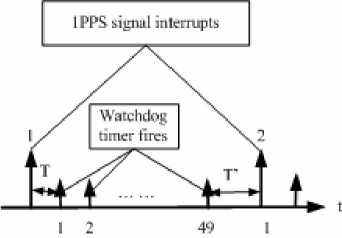
Figure 3 watch dog timer in repeated mode

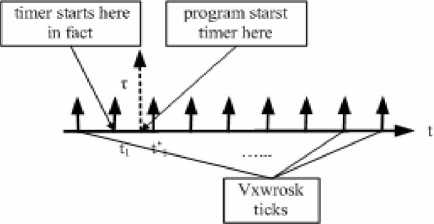
Figure 4 watch dog timer ~ time ticks

Vxworks). The result is that the real step time of the first watch dog timer contains an error of τ (Fig.4), this error τ can't be corrected at the next 1PPS interruption procedure, and the error would be cumulated to the tick period of Vxworks system. That is because of that the watch dog timer can only be started at the tick points, shown as the short arrowhead in Fig.4. In our project, the frequency of time ticks is set to 500, and so the error can only be corrected while it is cumulated to 2 milliseconds.

A much better resolution can be achieved by setting a higher frequency of the time ticks in Vxworks. But the system would be unstable and ineffective with too much frequently time tick interrupts. The frequency of time ticks is below 1KHZ under Vxworks systems usually, so the error can't be less than 1 ms.

A set of experiment data from watch dog mode is shown in Fig. 5. The sub step is set to 20 milliseconds here, and the points in figure indicate intervals measured for each sub step. Since the time measure function is from Vxworks with local crystal oscillator, the majorities are stable and equals to 20 milliseconds as assumed. The key point is when 1PPS signals arrive, the error between the local crystal oscillator and time server emerges. The local crystal oscillator is "faster" than the time server in our project, which means that real time of each sub step is actually a bit shorter. While the forty nine watch dog timers finish, 0.7 millisecond is added to the last sub step controlled by external 1PPS signal from the time server. That is why there is a value much larger than the majority every fifty points in Fig.5. The first watch dog timer stared by the 1PPS interruption procedure, as analyzed before, starts 0.7 milliseconds ahead of the programming time(0.7 is less than 2 millisecond and can't be adjusted), which induces that 0.7 millisecond is subtracted from the next sub step. The error is cumulated to about 1.3 millisecond on the next 1PPS signal shown in the figure, since it is also less than 2, the error can't be adjusted. When the error exceeds 2 milliseconds on the forth 1PPS signal's arriving, the time error of the first watch dog timer started by the forth 1PPS interruption procedure is reduced by a tick time (2 milliseconds).

timer must start at the time when time ticks are triggered in Vxworks. That is, we can see from Fig.4, although the program start a watch dog at time t1, it doesn't start exactly at t1, it starts actually at the previous tick time instead (The short arrowheads indicate the ticks in

watch dog mode

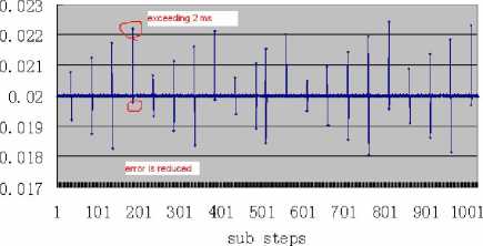
Figure 5 sub step times' variety under 1PPS signal

Since the error cumulates to 2 milliseconds, that is not satisfied for real-time simulation of navigation signal, the second method of PCI1780 counter mode is adopted. In this method, a counter on PCI card is used instead of the watch dog timer. For PCI1780, the clock onboard can be set with arbitrary frequency as needed (no more than 10MHZ). 50KHZ is chosen in our project, which means a much high resolution of 20 microseconds can be achieved. Comparing the 500HZ of the watch dog timer, it is much better and acceptable in our project.

D Time Synchronizat iin real-time model subsyste

There is only one computer in the real-time model subsystem that is installed with the PCI1780 card to synchronize with time server. This special computer is called as time router in real-time model subsystem. The other computers in the subsystem are synchronized with time router.

Simulation engine is designed to support parallel simulation of models and runs on each computer, including model computer and time router. Time synchronization is also done by the simulation engine, because simulation time’s advance is coherent with the simulation procedure. Since all the computers in realtime model subsystem are installed with RM 5565 node cards, time synchronization can be done through RM network: Time router is first triggered by the interrupt from PCI1780 at each simulation step, and then sends an special RM event through RM network to all the node cards. The other model computers are waiting for the event in the procedure of time synchronization, and continue to finish the work left in current simulation step on receiving the synchronization event from the time router, and then come to the waiting mode again for the next event. Because of the fast transportation and deterministic latency, time event sent by the time router can be checked within several microseconds, that is much better than time synchronization done by Ethernet, and is enough for real-time simulation with step of 20 milliseconds.

E Time Synchronization Logic under Disturbance

Besides the elements mentioned in the previous section, another factor may affect the effect of time synchronization. That is synthetic disturbance, which cost by circumstance and signal transportation.

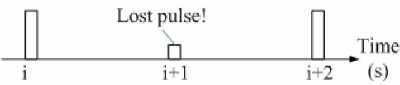
The first type of disturbance is signal’s lost. It is assumed that the 1PPS signals are sent exactly one per second. But for some reasons such as attenuation and disturbance or jamming from the environment, it is not always the case. Fig.6 zooms in and demonstrates the ascending part of the curve from the pulse signal, while Fig.7 gives the overall view of the 1PPS signals. Fig.6 (a) is a perfect waveform of the ascending curve, which trigger just one interrupt at each ascending moment. (3.3V is the typical TTL high level of input voltage). Waveform of Fig.6 (b), on the contrary, goes up slowly for the attenuation, and can not rise to the high level voltage of 2.4V. So no interrupt is triggered, which may slow down the time advancement of the simulation

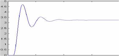
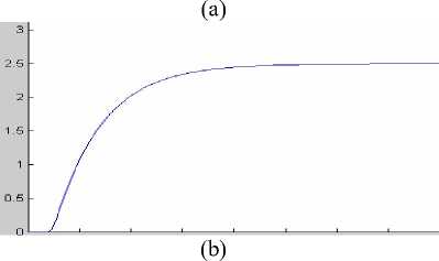
Figure 6 ascending curve of 1PPS signal

(a )

(b)

(c)

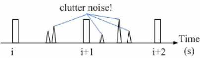
Figure 7 overall view of IPPS signals computer. Fig.7 (a, b) present a bird's-eye view of the two kind of waveforms. Fig.7(c) illustrates another phenomenon which is brought by the jamming noise from the environment, and these noises may cause chaos in 1PPS signals.

Lost of signal and jamming noise signal, these two kinds of disturbance must be done with to get successful synchronization.

To cope with the lost of signal, a watching timer is created at each 1PPS signal by ISR. The interval of the timer is one second plus δT 1 . If the next 1PPS signal comes on time, the ISR kills the previous watching timer and creates a new one; if the next 1PPS signal is lost on the contrary, the watching timer would be triggered at the time δT 1 past one second to give alarm. The interval of the watching timer, δT 1 should be chosen carefully. If it is too small, the timer would be triggered before the correct 1PPS signal, and it would bring much larger error while it is too large. The choice of the interval is depend of the local timer’s precision, for common computer, one

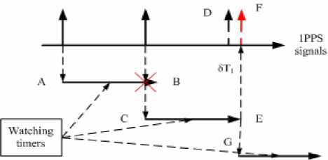
Figure 8 Lost 1PPS signal checking millisecond would be a reasonable choice.

Fig.8 illustrates the logic method to handle with the lost 1PPS signal:

• i)    A watching timer is created at each 1PPS signal (A), and the time interval is a bit longer than one second (B).

• ii)    If the next 1PPS signal comes at time, it would delete the previous timer (B), and create a new timer(C).

• iii)    If the next 1PPS signal is lost (D), the watching timer would not be deleted and fire at time δT 1 past one second (E), and a simulated interrupt is triggered (F), which calls the ISR as a normal interrupt. A new watching timer is created as normal (G).

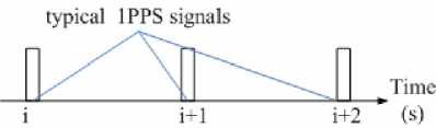
As to the second type of disturbance, jamming noise signal, a check procedure is adopted. While a signal (noise or 1PPS) comes, an interrupt is triggered as the standard 1PPS signal, the ISR measures the interval between it and the previous 1PPS signal. If the interval is within one second minus δT 2 , it is considered as a noise signal and is ignored.

Fig.9 gives an overall view of the logic: P is the standard 1PPS signal, while P 1 and P 2 represent the lost signal checking and noise signal checking points respectively, and the short arrows represent the noise signals. δT 1 is the lost signal checking boundary and δT 2 is the noise checking boundary. If the noise signal comes between P 2 and P, it would be considered as a valid 1PPS signal. If the noise signal comes before P2, it is treated as noise and abandoned. δT 2 , like δT 1 , must be also chosen carefully. If it is too small, a valid 1PPS signal would be treated as noise signal because of the time error between the local crystal oscillator and the standard one, and if it is too large, it would increase the probability which noise signal is confused with standard 1PPS signal. In our system, one millisecond is chosen as δT 2 .

Although it is seldom that the noise signal comes between P 2 and P, it is occurred by chance, and the logic method must think of it and adjust to it. Another checking

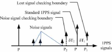
Figure 9 checking logic according disturbance routine is created to measure each “noise” signal, if the intervals of three adjacent “noise” signals are approximately equal to one second, these series signals are admitted as valid standard 1PPS signals and the logic is adjusted.

There are so many elements in the time synchronization, which bring time synchronization error: The latency of the interrupt service routine, the local timer granularity and error, the software programming and the synthetic disturbance are all combined together. How do these elements influence the time error? It’s hard to give a precisely analytic answer, so an useful method to study this issue is simulation.

W CONSTRUCTING OF SIMULATION MODELS

In order to study the time synchronization method, simulation method is considered as a valid tool, and Arena simulation software is adopted.

Arena is developed from the early SIMAN/CINEMA simulation software by Rockwell Software, Inc. It is an easy-to-use, powerful tool that allows you to create and run experiments on models of your systems.

In order to simulate the time synchronization in Arena, some models need to be constructed at first.

A Time Source Model

Time source is the basic element in time synchronization system. There are two kinds of time source in our system, one is the standard time source and the other is the local time source.

For standard time source, there are also two kinds: The first is 1PPS signal source and the other is sub-step time source with step of 20 milliseconds. Since there are no signal components in Arena, we use the “Create” component instead. 1PPS signal is sent from the time source, it is simulated as an entity, so “Entity” component is adopted in model.

It is the same for the local time source model, but the time interval parameter is different: a value of g_ticksDelt is introduced as the time error with the standard time source. In our system the time source is considered as constant in the simulation, so a constant value is used in the model.

B Signal Transportation Model

1PPS signals are transferred through physical link cable. It is simulated by “delay” component in Arena, and named as “Environment”. Assuming signal is transported by cable with length of 30 meters, transport delay is about 0.1 microseconds. The 1PPS signal entity is sent into the Environment component and delayed about 0.1 us, and then sent out to the next component.

C Software Delay Model

1PPS signal is sent to the time card installed on time router, and it would rely on the software routine to handle with this signal. The software routine must cost time to process the logic and bring error to the time synchronization obviously. So the software delay must be taken into account and be modeled in Arena.

Compared with the transportation delay, software delay is much more complex. There are two methods to handle the 1PPS signal in software. The first is query method, that is, a counter is used to count the incoming 1PPS signals, and software routine checks counter repeatedly. If a new signal come, the counter would increase its value by one, and the software routine would detect the increase at the next checking. This method is easy and simple, and the checking delay time is about a few microseconds, but it would add extra burden to CPU and PCI bus, so it is seldom adopted in fact. Another method is interrupt method, which means, an interrupt is triggered on each incoming signal. In this method, the time delay is dependent on the interrupt response, which relies mostly on the target operating system. If ordinary windows system is chosen as the target operating system, the message passing process would cost milliseconds of time delay, and what’s more, the delay would be variable from several milliseconds to hundreds of milliseconds, which bring much more difficulties and abnormal error in time synchronization. So in order to reduce the time delay and variation, a specific real time operating system, Vxworks, is applied in the distributed time synchronization. In Vxworks system, interrupt time delay is short and stable, which is about 2 microseconds (max: 2.76us, min: 1.86us), and the semaphore operating time is restricted within 200 nanoseconds [1], which are much better than in windows system.

“Delay” component is used to simulate the software delay in Arena. The delay time is not constant as the previous “Environment” model in Arena delay component, but is assumed as triangular distribution instead.

D Disturbance Model

The first kind of disturbance, lost of signal is modeled by “Decide” component in Arena. When 1PPS signals are passed to the decide component, probability calculation is done by Arena simulation engine, most of them are transferred to the next component and some of the signals are discarded to another route, which produce the lost of the signals. The probability of the lost can be set in the component.

Another kind of disturbance, noise signals, can be modeled by “Create” component like the time source model. The noise signals are also simulated as entities and combined with the normal 1PPS signal entities. The time distribution of noise signals is of random type (Expo in Arena), not constant like the normal time source.

E Synchronization Logic Model

From the previous section, we know that the logic to handle with the synthetic disturbance is complex, involving measurement and logic decision, this logic can be modeled by Arena. In order to restrict the paper length, the Arena model outline is put forth as Fig.10 without detailed description.

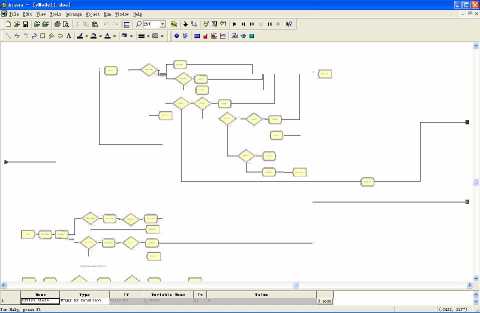
Figure 10. Synchronization Logic model in Arena

V SIMULATION AND ANALYZATION

From the previous analyses, the whole model of the time synchronization can be constructed with Arena (Fig.11). The subsystem of “External ISR” in the central part of the model is the key component, which is expanded in Fig.10. Some global variables are displayed on the left part of the model, which shows the key value during the simulation process. The time synchronization error values are recorded to the file, and can be analyzed after the simulation.

Time synchronization under synthetic disturbance simulation is done under these conditions: sub-step interval is 20 milliseconds; noise signal’s interval is accord with random distribution having mean value of 4.3 seconds; relative time error of local time source is of 0.01%; the granularity of the local time source is of 20 microseconds. During the simulation, local time values are measured with standard time source and recorded at each sub step.

Fig.12 is the result with no synthetic disturbance. Compared with standard time, local sub step intervals keep stable, and the max time error is less than 150 microseconds. Fig.13 gives the result with synthetic disturbance. Since there are disturbances, the initializing of time synchronization is longer than normal. (So, data number in Fig.13 is less than number in Fig.12). But once the initialization is done successfully, the sub step intervals also keep stable, and the time synchronization errors keep close to those with no disturbance. The simulation results prove the efficiency of the synchronization logic under synthetic disturbance.

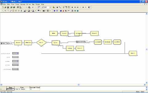
Figure11. Synchronization model in Arena

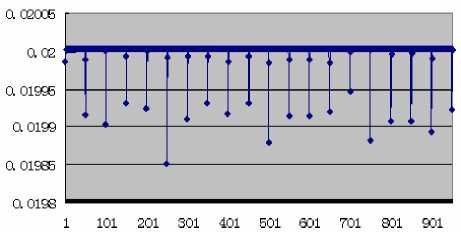
Figure 12. Synchronization with no disturbance

Cl 02002 ---

0l 02                                          ---------------------

0l 01998                      ^{:   :}— ^ -----------------------i

Q 01996 --------------1

Q 01994.-------------- a 01992 --- i---1*11--

0. 0199---------------- ----------------------

Q 01988 —------------------------------------

Cx 01906 ---------------------------------------------------------

CX 01984. -------------------------------------------------------------- a 01982                                                           1

1   101 201 301 401 501 601 701 801 901 1001

Figure13. Synchronization with disturbance

№ Summary and prospect

Distributed simulation system of satellite navigation signal is introduced, and synthetic disturbances are analyzed in the procedure of time synchronization in the system under 1PPS signals. A combined time synchronization method with 1PPS and SNTP is studied under synthetic disturbance, and Arena software is chosen as a software tool to study the procedure. The main parts of the synchronization system are modeled by Arena and whole simulation system is constructed, results of the simulation are put forth in the end. The simulation results show that the time synchronization logic is valid and the Arena software is competent for the studying of time synchronization methods.

One point should be mentioned is that the simulation speed of Arena. Since Arena is a discrete simulation software, the basic simulation step is dependent of the least time interval of the system. In our experiment, the least time interval is 20 microseconds, which is the granularity of the local time source. With this step time, the simulation speeds up is at about 0.1 with the real time on a 1.6G CPU computer. That is, simulation of procedure of 20 seconds would run about 200 seconds in fact. If the granularity is reduced, the simulation would be much slower. In order to get faster simulation, new simulation and modeling methods must be studied.

A CKNOWLEDGMENT

This work was supported in part by a grant from the National Natural Science Foundation of China (Grant No. 61074108).