Torsion of prismatic orthotropic elastoplastic rods

Introduction. Conservation laws were introduced into the theory of differential equations by E. Neter more than 100 years ago and are gradually becoming an important tool for the study of differential equation systems. Not only do they allow you to qualitatively investigate equations, but, as the authors of this article show, they allow us to find accurate solutions to boundary value problems. For the equations of isotropic theory of elasticity, the laws of preservation were first calculated by P. Olver. For the equations of the theory of plasticity in a two-dimensional case, the laws of preservation are found by one of the authors of this article and used to solve the main boundary value problems. Later it turned out that the laws of preservation can be used to find boundaries between elastic and plastic zones in twisted rods, plates and curved beams. It is assumed that the remaining current depends linearly on the voltage tensor component. As a result, an endless series of conservation laws have been found, which allows us to find the elastic boundary that arises when the orthotrope rod is twisted.

Problem setting . Consider an elastic orthotropic prismatic rod with an arbitrary cross-section. The side surface is stress-free, and forces equivalent to a torque of M are applied to the ends.

Let the origin be at the center of gravity of the end section, and the z-axis be parallel to the generatrix of the rod. The boundary conditions are written as follows:

° J + Ту m = о, xxy

Т xyl + ° ym = 0,(1)

Т xzl + Т yzm = 0, and on the ends of the rod (z = 0, z = l)

jj т xzdxdy = 0, jj т yzdxdy = 0, nn jj о zdxdy = 0, jj x о zdxdy = 0,

n          n

jj y о zd:xidy = 0, n jj(x Т yz - у Т xz) dxdy = M, n where n is a cross-section.

As usual in the theory of torsion, we believe that

° x  ° y   ^Т xy ⁰,

The rest of the stress tensor components satisfy the equilibrium equations, which will be written as follows:

dT     _n ^dT yz _а

—xz — 0,—— — 0, dzd

9txz   dT yz xz +  y_ +   z = 0.

dx    dy

Guk's generalized law for orthotropic environments will be written as follows [16].

dw  du         dw dw

.

аз Ozz = —

33 zz dz

a= t_xz = — + —, ад Tvz = — + —

55 xz44 dx  dz           dy a is an elastic constant here.

From the equations of joint deformations we get a13

^a 23

d 2 ° z	d 2 ° z		d 2	° z	d 2 ° z
d x 2	dy 2		d z 2		d x d y
d 2	d	i	a 44	d	T yz + a 55
d y d z ° z	d x	к		d x
5 2 c	d		— a 55	d	T xz + a 44
d x d z ° z	d y	к		d y

= 0,

a

T- ^T xz

,

d_   )

TI .

d x ^y J

From (6) and boundary conditions (1) we obtain that ° _z = 0 in all cross-sections.

Of the last two equations (6) it follows (6)

d         d

~a 44 — ^T yz ⁺ a 55    ^T xz = const.

d x         d y

Since

a 55 ^T xz

a 44 ^T yz

dwd

= dx dwd

= , dy

then we have

d

d

a 55    ^T_Y_    a 44    ^T_v-

55      xz    44      yz dy        dx

did u   d v

—

d z к d y   d x

— 2 ^^ z = — 2 0 . d z

where to z is the third component of the vector rot ( u , v , w ) . Therefore 0 is a corner of twisting, per unit of length. It's called a twist.

The problem of elastic torsion of the prism rod was reduced to the integration of equations.

^dT xz , ^dT yz _ о _n ^dT xz _     ^дт yz _

+     — 0, a^       адд     —  20, dx    dy        55 dy    44 dx and the boundary condition tyД + t. mt = 0. xz     yz

It is easy to see that the system of equations (8) is reduced to a linear equation of the second order of the elliptical type.

In the plastic area, the equations (8) should be added to the condition of plasticity, which has the following form:

^{2 a} 13 ^T xz ^{+ 2 a} 23 ^T yz = ^1.

Here a3, a23 are the constatnts, characterizing the current state of plastic anisotropy.

The result is the following task: to find conservation laws for equations (8) that allow you to solve the problem (9). These laws will find a boundary between elastic and plastic areas.

Conservation laws for orthotropic elasticity equations . This part will provide conservation laws for equations (8) to be used further to solve elastic problems.

For simplicity of further layouts, we will write down the system (8) in the form of:

F 1 = u x ⁺ v y ^- f ¹ = 0,

F2 = aUy-вVy - f2 = 0, where u = txz, v = t , a = a55, в = a44 , the index at the bottom denotes a derivative on the corresponding variable.

Let's call the vector ( A , B ) as a persistence current for equations (10) if

A x + B y =П 1 ( F ) + П 2 ( F 2 ) = 0,                             (11)

executed on all smooth system solutions (11). Here Пг are some non-identical linear differential operators.

In this case (11) is the law of preservation for the system (10).

Let's set a task to find the laws of preservation for (10) if the remaining current depends only on x , y , u , v .

Note. Nothing also prevents us from finding conservation laws with a persistence current dependent on any number of derivatives, but we will limit ourselves to these, since other conservation laws have not been used for boundary problems yet.

Let

A = a u + в v + y , B = a u + в v + y , where ai, вi, уi are the functions only from x, y

Of (11) we have

a u + a u + вгv + в Vx + Yv + avu + a u + вVv + в Vv + Yv = x    xx    xx  y    yy    yy

= 8 1 ( u x ^{+ V}y — ^{f 1} ) + S ² ( ^a u y ^{-в V}x — ^{f 2} ) .

From (13) we get ax + ay = 0, вX +в; = 0, a1 =в2 =81,в1 = -82в, a 2 = 82a, yx + yyy = -81f 1 - 82f2,в^ = - a2/.

Finally we have

a ! + a У = 0, ^ва 2 -a y = 0, y ! ⁺ У 2 = ^-a ¹ f ^{1 -} — f ² a                      a

For simplicity we consider that у ² = 0. Then we get:

a1 =U2, р1=-ва2, у1    |  ■ f1 -52 f1a        J        a

dx

and the coefficienst a¹ and a ² are linked by equations:

a ! + a ² = 0, Pa 2 - aa ^ = 0.

We find two special solutions to this system. They have the following form.

First solution:

a1 =

x

a 2

Second solution:

a 2

x

For the simplicity of further calculations, let's put у = a 4y   = q .

'    / ^a     / ^a 55   "

Next, we note that equation (16) admits following symmetries

! ‘ = ! + ! о , у ‘ = у + у о , where x0, y0- are arbitrary constants.

Therefore, the obtained solutions can be written as:

_a 1 =         ^{! - !} o         , _a 2 =         у ^- У о        ,

( ^{! - !} o ) ² + q ( у ^- у o ) ²         ( ^{! - !} o ) ² + q ( у ^- у o ) 2

_a 1 =-       ^{q ( У} - ^у 0 )       , _a 2 =        ^{! - !} o

( ^{! - !} o ) ² + q ( у ^- у o ) ²        ( ! ^- ! o ) 2 + q ( у ^- y o ) 2

We obtain two remaining currents.

A = ^{a 1} u ^- q ^{a 2} v ⁺ у ¹, B i = ^{a 2} u ^{+ a} * v , then, two conservation laws are obtained

From (19) we get:

d, a +d_y в = o.

xy

[^ Ady - B i d! = 0,

Г

where Г₁ is the contour that does not cover the point ( ! ₀, у ₀ ) .

Now let the point ( x₀, y 0 ) lie inside the region D, the boundary of which is the contour Г . In this case, the formula (20) can not be applied directly. Therefore, we use the standard technique: we describe an ellipse around the point of the following form: ( x - x ₀ ) 2 + q ( y - y ₀ ) 2 = 8 2 (Fig. 1).

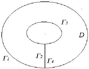
Рис. 1. Вычисление контурного интеграла вокруг особой точки

Fig. 1. Calculation of the contour integral around a singular point

Let's denote this ellipse Г1 . Then we can easily get

[J Ady - B i dx = -[J ( A i dy - B i dx ) , ГГ

We calculate the integral in the right part of formula (21) for i = 1,2 .

Let i = 1. We have:

Г 1 Г 1

( ^{x - x} 0 )

i ( ^{x - x} 0 ) ² + q ( y - y 0 ) ²

q (y - y о )

( ^x - ^x 0 ) ² + q ( y ^- y 0 ) ²

V ⁺ y 1

dy -

( y ^- y 0 )

_v ( ^x - ^x o ) ^{2 +} q ( y ^- y о ) 2

( ^{x - x} o )

( ^{x - x} o ) ² + q ( y - y o ) ²

v dx =

^f ( ^{x - x} o )

q (y - yo)

V ⁺ Y i

,   f ( y - y0 )

dy - -—r^ l ⁸

( x - xo) L

-—т-^ V dx.

8     7

Let’s introduce the notation x - x ₀ =8 cos 6 , y - y ₀ =8 sin 6 .

So we have:

sin 2 6

qu - ( 1 - q )

2n v + y1 I d6 = q J u (x0 +8 cos 6, y0 +8 sin 6)d6.

⁷         0

In the resulting expression, we aim at zero and, using the mean theorem, we get

[J = ^{2 n} qu ( x o , y o ) .

Г 1

Now from formula (21) we have

2 n qu ( x ₀, y ₀ ) = - J A 1 dy - B 1 dx .

Г

Let's consider the case i = 2. Similarly, we get:

^— q ( y ^— y о )

Г Г ( ( x ^— x 0 ) ⁺ q ^{( y — y} 0 )

u

—

q ( x ^— x о )

( x ^— x 0

) ² + q ( y ^— y о ) ²

^{v +} y 2   dy

—

=^

Г 1 ^V

(x—xo)

v ( x ^— x o ) ² + q ( y ^— y о ) ²

q (y—yо)

( x ^— x ) 2 + q ( y ^— y о ) 2

v dx =

q (y—yо)

u

q ( x ^{— х} о ) E 2

^

V + y 2   dy

—

^{f (} x ^— x о ) u - q ⁽ y - y о ) ^v )

V

E ²

dx

We enter the coordinates

x — x₀ =E cos 6 , y — y 0 =E sin 6 .

Now we have

(—q +1) sin 26

u

— qv

d 6 =

2 n

= — q J v ( x₀ +e cos 6 , y 0 +E sin 6 ) d 6 = — 2 n v ( x 0 , y 0 ) q .

Now we specify these conservation laws to twist the prism rod.

We have

^{2 n} q ^T xz ( ^x 0 , y 0 ) = [J ( ^a 1 ^T xz ^— q ^a 2 ^T yz + ^{2 6} J ^a 1 ^dx ) ^{dx —} ( ^a 2 ^T xz ^+a 1 ^T yz ) dy , Г

^{2 n} q ^T yz ( ^x 0 , y 0 ) = [J ( « 2 ^T xz ^— q ^a 2 ^T yz ^{+ 2 6} J ^a 2 ^dx ) ^{dx —} ( ^{a 2 T} xz ^+a 2 ^T yz ) dy . Г

Elastic-plastic boundary in a twisted rectilinear orthotropic rod .

Consider the elastic torsion of the orthotropic straight rod, the cross-section of which is limited by the convex outline of Г.

At a fairly high value of torque, the rod forms an elastic F zone and a P plastic zone (Figure 2).

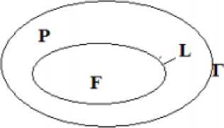
Рис. 2. Поперечное сечение скручиваемого стержня

Fig. 2. Cross-section of the twisted rod

It is known that the plastic zone begins to form on the outer contour of Г . Suppose that the plastic zone completely covers the outer contour. Let L be the boundary of the division of elastic and plastic zones.

The purpose of this paragraph is to build the L border in an explicit form with the help of conservation laws built in previous paragraphs.

Problem setting . In the elastic zone, the stress tensor components satisfy equations (8)

^дт xz . ^dT yz _₀  „   ^дт xz _ -   ^dT yz __26

+        0, a^c        алл          2U, дx    dy       55 дy    44 дx

on the outer contour Г to the boundary condition

and the condition of plasticity

т_. д +т m — о. xz      yz

^{2 a} 13 ^T 2 z ^{+ 2 a} 23 ^т 2 z ^— 1 -

From ratios (27) --28) you can identify the components of the tensor т _xz , т _yz on the Г contour.

We have now

m

2 a ₁₃ m ² + 2 a ₂₃ 1 ²

^т yz lr

l

2 a ₁₃ m ² + 2 a ₂₃ l²

Here the signs are chosen according to the torque (3).

In (24) we receive the following conservation laws.

^{2 n} q ^т xz ( x o , y о ) ^— -J A i dy - B i dx ,

Г

и

^{2 n} q ^т yz ( ^x 0 , y 0 ) ^— - J A 2 dy - B 2 ^dx .

Г

To calculate т _xz ( x ₀, y ₀ ) and т _yz ( x ₀ , y ₀ ) we use formulas (29)-(30). From these formulas we get т _xz and т _yz at all points inside the rod. Now let's check the condition (27).

At those points where the expression in the first part (27) less than one will fall into the elastic zone, and the rest of the dots in the plastic.

Conclusion . These calculations allow us to restore the desired boundary of L. with any accuracy. For the isotropic case, this problem was solved for the first time in [12; 14]. Examples of constructing elastic-plastic boundaries for different types of rolled profiles are considered in [10].