Translation movement stability control of quad tiltrotor using LQR and LQG

Author: Andi Dharmawan, Ahmad Ashari, Agfianto Eko Putra
Journal: International Journal of Intelligent Systems and Applications @ijisa
Article in issue: 3 vol.10, 2018.
Free access
Quadrotor as one type of UAV (Unmanned Aerial Vehicle) is a system that underactuated. It means that the system has a signal control amount is lower than the degrees of freedom or DOF (Degree Of Freedom). This condition causes the quadrotor have limited mobility. If quadrotor is made to have 6 DOF or more (overactuated system), the motion control system to optimise the flight will be different from before. We need to develop overactuated quadrotor control. Quadtiltrotor as the development of quadrotor has some control signal over its DOF. So we call it as an overactuated system. Based on the type of manoeuvre to do, the transition process when the quad tiltrotor performs a translational motion using the tilting rotor need special treatment. The tilt angle change is intended that the quad tiltrotor can perform translational motion while still maintaining its orientation angle near 0°. This orientation angle can change during the undesirable rotational movement as the effect of the transition process. If additional rotational movements cannot be damped, the quad tiltrotor can experience multi overshoot, steady-state error, or even fall. Because of this matter, we need to develop flight control system to handle it. The flight control system of quad tiltrotor can be designed using a model of the system. Models can be created using quad tiltrotor dynamics by the Newton-Euler approach. Then the model is simulated along with the control system using the method of control. Several control methods can be utilised in a quad tiltrotor flight systems. However, with the implementation of LQG control method and Integrator, optimal translational control of the quad tiltrotor can be achieved.
UAV, quadrotor, overactuated, underactuated, Newton-Euler
Short address: https://sciup.org/15016467
IDR: 15016467 | DOI: 10.5815/ijisa.2018.03.02
Text of the scientific article Translation movement stability control of quad tiltrotor using LQR and LQG
Published Online March 2018 in MECS
UAV is defined as an unmanned aerial vehicle, using aerodynamic force to fly, either flying autonomously using an autopilot system or remote control. UAV is also known as UAS (Unmanned Aircraft System) [1]. UAVs have been developed for various purposes, such as having the ability to perform various types of sensing missions for civil or military to building monitoring [2]. The missions that can be implemented by the UAV consist of surveillance, reconnaissance, monitoring, air patrol, high-resolution aerial photography and so on [3].
UAVs have several types, such as rotary wing (multirotor), fixed wing, flapping wing (ornithopter), and blimp (air balloon). One type of UAV with a rotary wing type is a quadrotor [4]. The quadrotor is a multi-rotor type UAV that has four rotors (propellers).
The quadrotor is an underactuated mechanical system. That is a system that has some control signals less than the degrees of freedom (DOF) available [5]. In the quadrotor flight, there are control signals consisting of a thrust, torque for rolling, torque for pitch motion, and torque for motion yaw [6]. On the other hand, the quadrotor is required to manoeuvre with 6 degrees of freedom, which consists of translational motion along the x, y, and z-axes and rotational motion consisting of a roll, pitch, and yaw motion. The underactuated quadrotor design limits its flying manoeuvrability and also decreases the likelihood of interacting with the environment by exerting desired forces in a more free direction [7].
Motivated by this consideration, several solutions have been proposed in previous studies covering different concepts, such as the tilting-wings mechanism [8], UAVs with non-parallel lift [9], or implementing Tilting-rotor [10].
Quadtiltrotor as the development of quadrotor has full 6 DOF motion [11]. It uses frames with (+) flight configuration of the modified quadrotor by adding servo motors on each end of the arm which is the rotor position so that it can be tilting. When the vehicle successfully reaches the full 6 DOF motion, the control system to optimise the flying motion of the vehicle becomes different from before. One of them that needs to be optimised is the attitude control of the quad tiltrotor when hovering. It is due to the increasing number of motion manoeuvres that can also be performed proportionally to the amount of interference received.
Based on the type of manoeuvre that can be done, the transition from quad tiltrotor to hovering to translational motion is a matter of concern. The translational motion is performed by involving a tilt angle change from the rotor on an axis. This angle change aims to allow the quad tiltrotor to perform translational motion while maintaining its orientation angle. This orientation angle consists of roll angle, pitch, and yaw. This orientation angle changes when unwanted rotation motion occurs as a result of the transition process. Furthermore, the transition from translational motion back to hovering state also needs attention [12]. If the transition process does not work properly, such as the emergence of additional unwanted rotation movements, it may cause the vehicle to experience multi overshoot, unfocused flight (caused by a significant steady-state error), or even fall.
Multi overshoot and steady state errors can appear in a various state of the system. They will lead to irregularities in the quad-tiltrotor flight, so it needs to be handled properly [13]. Therefore it is necessary to adjust the control system so that optimal conditions are obtained, such as no multi overshoot, small overshoot, minimum steady state error, as well as adequate rise time and settling time.
Various control methods have been offered to address the problem. Some researchers have tried to apply different types of flight control methods to an aircraft, in particular, the quadrotor series. They consist of PID (Proportional, Integral and Derivative) methods [14] [15], LQ (Linear Quadratic) [16] [17] [18], utilising fusion and filter methods such as complementary methods, DCM (Direct Cosine Matrix) filters, and the Kalman filter method [19]. LQ methods, such as LQR (Linear Quadratic Regulator) and LQG (Linear Quadratic Gaussian) utilising HJB (Hamilton-Jacobi-Bellman) equations in managing cost functions to achieve optimal control. The methods and algorithms have their respective advantages and disadvantages. However, based on the characteristics and workings of these methods LQ methods can be implemented on a control system for aircraft [20].
LQR and LQG work in MIMO (Multiple Input Multiple Output) using state space as a representation of system model. LQG is a development of LQR utilising Kalman filters to generate state-controlled estimators, including overcoming white noise (Welch and Bishop, 2006). However, LQG which is the development of LQR is a method of control that is to maintain the value of a state in the position of zero. Therefore it is necessary to develop from LQR and LQG techniques so that the vehicle can fly under the desired reference.
This paper has a structure consisting of introduction, material and method, results and discussion, and conclusion. Material and method discussed quad tilt-rotor dynamics and all types of control methods used. The control methods consist of LQR, LQR and Integrator, and LQG. Results and discussion examine the results of the implementation of control methods and their respective comparisons. The paper then concludes with conclusions as well as future works.
-
II. The Material and Method
-
A. Quad Tiltrotor Dynamics
Quad Tiltrotor can be modelled as connections of the five main rigid bodies in relative movement between body B and 4 group propellers P i consisting of 4 motor arms to swing each propeller group. The propeller group itself is connected to each rotor (as shown in Fig.1).
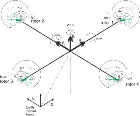
Fig.1. Configuration of earth inertial framework and quad tiltrotor body
E :{ OE; E x , E y , E z } is the earth's inertial framework and B: { OB; Bx, By, Bz } are the moving frames of the rides bodies at the centre of mass. In the quad tiltrotor model, there is Pi: { OPi; Pix, Piy, Piz } ( i = 1...4) defined as the frame connected to the i -th propeller group as shown in Fig.2.
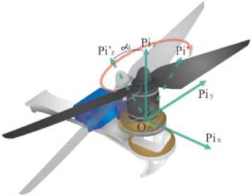
Fig.2. The i -th swinging arm visualises the body frame P , propellers associated with lifting force F , and the angle of swinging propellers α
Rg will represent the orientation of the body frame B to the earth frame E based on rotation matrix [21], while the Rp. denotes the orientation of the group of i -th propeller frames connected to the body frame. Using the
∈ ℝ as the propeller swing angle to the P ix -axis and Fig.2 as the visualisation of rotation of the propeller group P i on the body frame, we obtain the equation (1).
=
=( - ) + +
̈=( - ) + + where
= (( -1) ) ( ), =1,…,4․ (1)
=
=( - ) + +
̈=( - ) + + (5)
(α )=[0 сοs-sin
0 sinсοs
[сοs -sin0
sin сοs0
is the tilt angle of the i-th propeller group and γ = (i-1) . as the centre point of the propeller group frame Pi in body frame with is the distance between with (quad tiltrotor arm) shown in the equation (3) [11].
= (( -1) )[0] , =1,…,4
Then by utilising the Newton-Euler concept, we can obtain the dynamics of quad-tiltrotor motion in translation and rotation motion. The dynamics of quadtiltrotor translational movement are shown in the equation (4) [22].
-
• = , =1, 2, 3, 4
-
•
̈=
̈ =()
-
•
̈=
̈=( +)
-
•
Ez
̈=-
̈=( )-
F i is the thrust of the i -th rotor. b is the thrust constant of the rotor [23]. m is the total mass of the quad tiltrotor. (D i is the rotational speed of the i -th rotor. F Tx is the translational force along the x -axis. F Ty is the translational force along the y -axis. FTz is the force translations along the z -axis.
Then the dynamics of quad-tiltrotor rotational motion are shown in the equation (5).
= , =1, 2, 3, 4
=
= - + -+
- +-
̈= - + -+
- +-
T i is the torque of i -th rotor. k is the drag constant of the rotor[23]. m is the total mass of the quad tiltrotor. (D i is the rotational speed of the i -th rotor. Т ф is the rotational torque around the x -axis. t g is the rotational torque around the y -axis. tv is the rotational torque around the z -axis.
-
B. LQR Methods
We can use various methods to control a quad tilt-rotor. However, we can improve the control by implementing modern control system. Modern control systems use the concept of state space as shown in equation (6).
̇= +
= +
where
= state
= process input
= process output
= state derivative and state relation matrix
= state derivative and process input relation matrix
= output process and state relation matrix
= output and input process relation matrix
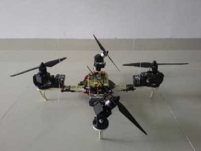
Fig.3. Prototype of quad tiltrotor
By using the modelling of the equations (4) representing the movement of translation in the x, y, and z respectively, we can tune create a state space model system of quad tiltrotor. Similarly, for rotation motion, we can use equation (5). By utilising a quad tilt-rotor prototype shown in Fig.3, we can simulate by filling entire components of these equations using the original data from the prototype.
We can apply control method on systems that have more than one input and output of each (MIMO or Multi Input Multi Output), like LQR (Linear Quadratic Regulator). It will be advantages if we compare to classical control methods such as PID control method that can only process a single input and a single output (SISO). PID control system can still handle the MIMO system, but we do it sequentially [24]. By changing the equation model (4) representing the movement of translation in the x , y , and z -axes respectively and the equation (5) representing the roll, pitch, and yaw rotation motion, we can make the state space equation as shown in (7)-(11).
By using the concept of full state feedback [25] [26], we can design a close loop control in state space system. Then we apply this concept by using K as feedback gain [20].
=
сοs V' сοs 9
=
сοs ф сοs Ф +sin Ф sin 9 sin Ф
сοs ф сοs 9
ГХ1
⎢⎡ Vx ⎤
У Vy
⎢ z ⎥
Шф 0 toe Ф .^ф.
=
⎢⎢⎢ I ⎥⎥⎥
⎣ ⎦ гУ1] ⎢⎡ y2 ⎤ ⎢ Уз ⎥ ⎢ ⎥ ⎢ У5 ⎥ ⎣ ⎦
where
=
0
1 0
0
0
=
0
0
0
0
U^ =(<^i sin «2 + шХ sin «4 )
U2 =( toX sin «1 + ti| sin «3 )
u3 =( toX сοs «! + ti| сοs «3 + «>x сοs «2 + toX сοs «4 )
U4 = (<^i сοs «2 - toX сοs a4)+к(coX sin «2 + toX sin a4 )
Wg = (
toX
сοs «4 -
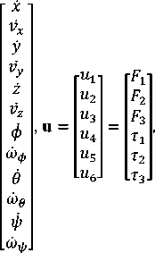
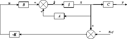
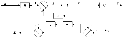
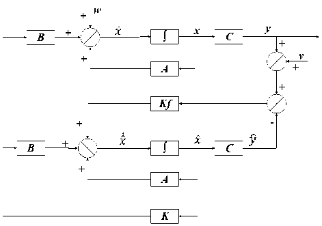
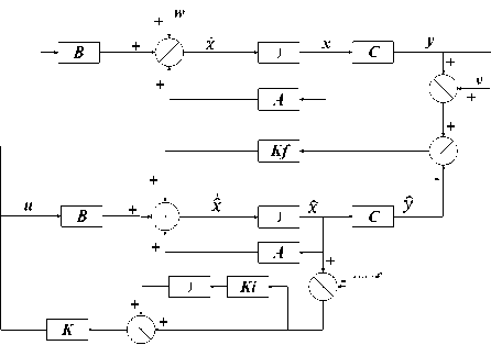
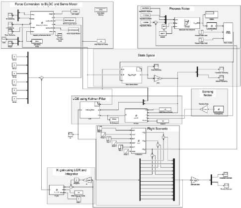
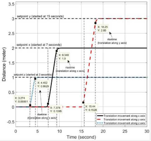
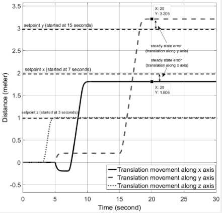
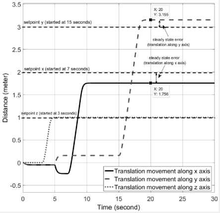
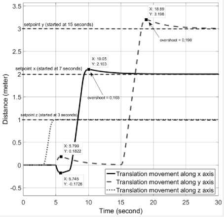
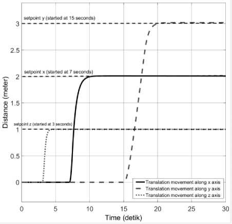
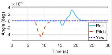
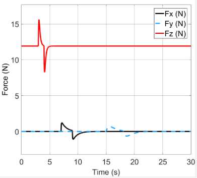
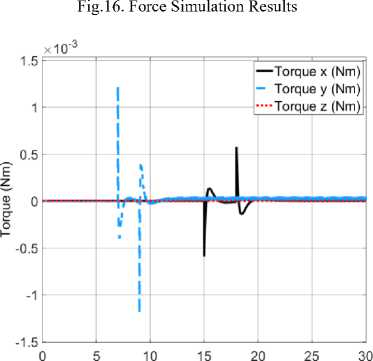
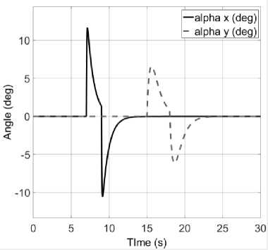
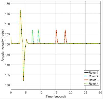
it6 =(toX сοs «1 - «>X сοs «2 + = 0 1 0 0 0 0 0 0 0 0 0 0 ⎢⎡0 0 0 0 0 0 0 0 “3 m 0 0 0⎤ ⎢0 0 0 1 0 0 0 0 0 0 0 0 ⎢0 0 0 0 0 0 “3 - m 0 0 0 0 0 ⎢0 0 0 0 0 1 0 0 0 0 0 0 ⎢0 0 0 0 0 0 0 0 0 0 0 0 (8) ⎢0 0 0 0 0 0 0 1 0 0 0 0 ⎢0 0 0 0 0 0 0 0 0 0 0 0 ⎢0 0 0 0 0 0 0 0 0 1 0 0 ⎢0 0 0 0 0 0 0 0 0 0 0 0 ⎢0 0 0 0 0 0 0 0 0 0 0 1 ⎣0 0 0 0 0 0 0 0 0 0 0 0⎦ Before we calculate the K gain, we design the control simulation using the concept of full state feedback in state space system as shown in Fig. K gain can act as the performance regulator matrix of the system. Input process feedback is influenced by K gain as shown in equation (12). и=-Kx (12) Fig.4. Control system design with K gain [27] -Ul ll2 1․11․2 2․12․2 3․13․2 4․14․2 5․15․2 6․16․2 1․3 1․4 1․5 1․6 2․3 2․4 2․5 2․6 3․3 3․4 3․5 3․6 4․3 4․4 4․5 4․6 5․3 5․4 5․5 5․6 6․3 6․4 6․5 6․6 1․7 1․8 1․9 1․10 1․11 1․12 2․7 2․8 2․9 2․10 2․11 2․12 3․7 3․8 3․9 3․10 3․11 3․12 4․7 4․8 4․9 4․10 4․11 4․12 5․7 5․8 5․9 5․10 5․11 5․12 6․7 6․8 6․9 6․10 6․11 6․12 у "z Ф «ф «« Specifically, this system uses the Linear Quadratic Controller (LQR) method to determine the control gain K on the state feedback. In this approach, we use two parameters Q and R that play a role in balancing the system stability of the control signal u and error (deviation from 0) to an optimal control system. The main idea in LQR control design is to minimise the cost function J shown in (13). № J=J (xTQx + uTRu) dt (13) t0 Regardless of the values of Q and R, we can obtain the cost function by solving the Riccati Algebra Equation (Algebraic Riccati Equation) [28]. We use Q and R parameters as design parameters to condition state and control signals. The gain matrix K can be obtained using equation (14). = (14) where the matrix P is derived from Riccati equation according to equation (15). + - + = (15) We choose Q values to regulate the performance of the system process. The increase of elements of the Q matrix is directly proportional to the components of the gain K. Conversely, the growth of the matrix elements R is inversely proportional to the gain K. If the selection of the R value is large, then the feedback becomes less influential to the system. On the other hand, choosing value 1 for R means we do not want R to affect the control. The simplest way to determine the values of the elements of the matrices Q and R is by using equation (16). R = 1 = (16) We map the value of each element of the matrix Q as shown in equation (17). Then we determine the values of Q and R using equations (10) and (16), as shown in equation (18) [27]. = Г& 0 0 0 0 0 0 0 0 0 0 0 0 Qvx 0 0 0 0 0 0 0 0 0 0 ⎢0 0 Qy 0 0 0 0 0 0 0 0 0 ⎢0 0 0 Qvy 0 0 0 0 0 0 0 0 ⎥ ⎢0 0 0 0 Qz 0 0 0 0 0 0 0 ⎥ ⎢0 0 0 0 0 Q^z 0 0 0 0 0 0 ⎥ ⎢0 0 0 0 0 0 Qф 0 0 0 0 0 ⎥ (17) ⎢0 0 0 0 0 0 0 0 0 0 0 ⎥ ⎢0 0 0 0 0 0 0 0 Qe 0 0 0 ⎥ ⎢0 0 0 0 0 0 0 0 0 Q 0 0 ⎥ ⎢0 0 0 0 0 0 0 0 0 0 Qcd^ 0 ⎣0 0 0 0 0 0 0 0 0 0 0 ⎦ R = 1 = 1 0 0 0 0 0 0 0 0 0 0 0 ⎡0 0 0 0 0 0 0 0 0 0 0 0⎤ 0 0 1 0 0 0 0 0 0 0 0 0 0 0 0 0 0 0 0 0 0 0 0 0 0 0 0 0 1 0 0 0 0 0 0 0 ⎢0 0 0 0 0 0 0 0 0 0 0 0⎥ ⎢0 0 0 0 0 0 1 0 0 0 0 0⎥ (18) ⎢0 0 0 0 0 0 0 0 0 0 0 0⎥ ⎢0 0 0 0 0 0 0 0 1 0 0 0⎥ ⎢0 0 0 0 0 0 0 0 0 0 0 0⎥ ⎢0 0 0 0 0 0 0 0 0 0 1 0 ⎣0 0 0 0 0 0 0 0 0 0 0 0⎦ Linear Quadratic Controller (LQR) method is a method devoted as a regulator. The problem that arises on LQR is what if the user or the autonomous system wants to change the reference from the state directly. We can make reference changes, where the magnitudes of the process states are not equal to the magnitudes of the reference, using the state reference as shown in Fig.5. Fig.5. Full-state feedback control system with state reference The system can maintain zero conditions by adjusting the new reference. On a quad tiltrotor flight, this is very useful. For example when the quad tiltrotor wants to keep the altitude even though the desired altitude changes. The new state space equation as shown in equation (19) uses the control diagram in Fig.5. ̇=Ax +В(г-К(х- ^ref)) (19) у= C. LQR and Integrator A steady state error reduction is required on the control system to conform to the desired control requirement specification. Unlike the other design methods, with feedback from the output compared to the reference input to calculate the error, the full state feedback control of the entire state is fed back. But before we need to calculate the state error of each desired state, which is then multiplied by the gain of K, and use the new value as a reference to determine the control signal. We can reduce the steady state error by adding Ki gain constant after state error, as shown in Fig.6. Gain constant Ki is a matrix with the size of the number of state multiplying number of states. Gain matrix Ki acts as an integrator working on a state reference, and the result affects the control signal u. In this way, we can minimise the steady-state error, but not all elements in the Ki gain matrix have value. We can set Ki matrix element as shown in equation (20). Fig.6. The control system design with Ki as integrator = In the equation, we can see that from the 12 states, we only integrate the states in the odd rows and columns (1st, 3rd, 5th, 7th, 9th, and 11th). These states are not derivatives of other states. If the state derived from another state is integrated, then the Ki matrix will change to a proportional gain, thus having a function equal to the gain of K. Therefore of the 12 states, there are only six states that can be integrated. D. LQG Methods In control theory, Linear Quadratic Gaussian (LQG) is one of the most central areas of a primary control system. It involves an uncertain linear system that suffers further disturbances in the form of white Gaussian noise, incomplete state information (i.e., not all state variables are measured and available for feedback) and as a subject control for a quadratic cost. The LQG controller can optimise the control of the non-linear system that is interrupted [20]. The LQG controller is a combination of Kalman filter, the Linear Quadratic Estimator (LQE), with Linear Quadratic Controller (LQR). It can estimate the state laike using soft computing methods [29]. The principle of separation ensures that it can be designed and calculated independently. We can apply LQG control to LTI (Linear Time Invariant) and LTV (Linear Time Varying) systems. The equation (21) shows a linear time-invariant (LTI) Gaussian design model. ̇=Ах + Ви +W у=+V where w is process noise, and v is the sensing noise as shown in equation (22). Е{W(t)wT (т)} = QoS(t-т) Е{V(t)VT (т)}=R06(t-т) The state estimator ̂ is formed using the Kalman filter estimator as shown in equation (23). ̂̇ = ̂+ + ( - ̂) О= + PfAT + Qo - P^R^Pf Kf = where ̂ is the estimation of the output, Pf=E{XXT} is the steady state error covariance which as in LQR is obtained by solving the Riccati Algebraic Equation, and Q0 and R0 are the covariances of process interference and covariance of the measurement noise (w and v respectively). The optimum control is formed using the full state feedback gain matrix K determined by LQR, and the feedback state estimator ̂ as the output of the LQE shown in equation (24). u=r-Kx̂ (24) If r = 0, so the block diagram of LQG control is shown in Fig.7. The state reference as shown in Fig.5, allows the system to maintain conditions under zero by adjusting the new reference. Therefore, the control diagram illustrated in Fig.7 is transformed into a control diagram as shown in Fig.8. According to Fig.8, equation (24) is adjusted to equation (25) и=-К(( ̂-^ref)+∫Ki( ̂-^ref ) dt) (25) Then, by modifying the design of the control system with shown in Fig.5, the input of the gain K is changed to the estimator ̂ obtained from the LQE process and subtracted by the state reference and also with the integrator as shown in Fig.8. Fig.7. The LQG control system design u - xref Fig.8. The LQG control system design with state reference and integrator III. Results and Discussion We can create the simulation diagram block in tools like Simulink based on diagram block in Fig.8 and state space system that we have made before as shown in Fig.9. The simulation model is divided into four pieces parts, consisting of: • State space with full state feedback • Flight Scenario • Process Noises • Force and Torque Conversion to Brushless DC (BLDC) Motors and Servos Rotation The state space with full state feedback is the central part of the system. This section is designed using the model of equation (7) - (11). Then the flight scenario mission arrangement consists of setting the quad tiltrotor movement direction. Flight is regulated by 3-dimensional motion directions, specifically the x, y, and z-axes. Process noises contribute to give some white noise (interference) on the system. These disturbances are generated randomly but still in the range that we have determined at specified intervals. Force conversion to a brushless motor (BLDC) and servo rotations represents the performance of a vehicle based on the model that we have simulated. We can set the K gain matrix value using various methods. Some example of the methods are manual tuning, ANN [30], Pole Placement [31], Ackermann [32], LQR [17], etc. After getting the K gain matrix value as shown in equation (26), we can run the simulation. = 31․6 27․8 0 0 0 0 0 0 10․5 0․02 00 ⎡ 0 0 3․14 4․15 0 0 -5․81 -0․01 0 0 0 0 ⎢⎢ 0 0 0 0 100 25․4 0 0 0 0 0 0⎥ ⎢ 0 0 -0․41 -0․64 0 0 46․0 11․0 0 0 0 0⎥ ⎢0․99 1․12 0 0 0 0 0 0 46․3 11․0 0 0⎥ ⎣ 0 0 0 0 0 0 0 0 0 0 34․610․1⎦ Fig.9. Simulation using Simulink Fig.10 shows the quad tiltrotor translation movement along x, y, and z-axes based on the scenario that we have created before. There are no overshoots on each of the translation movement curves in the figure. It is because the system has not received interference, both process and sensing. Fig.10. Translation movement simulation results using LQR without noise When the quad tiltrotor gets a horizontal wind noise process, it shifts from the desired setpoint. The disturbance of the horizontal wind process has a motion speed of -0.543 m / sec on the x-axis of the earth (latitude axis) and of 0.573 m / sec on the earth's y-axis (longitude axis). The negative value of the direction velocity of the x-axis of the earth means that the wind moves from north to south (as opposed to the direction of motion of the rides). A positive value at the direction velocity of the earth's y-axis means the wind moves in the direction of the quad-tiltrotor motion. Fig.11. Translation movement simulation results using LQR with process noise Fig.12. Translation movement simulation results using LQR with process and sensing noise Fig.13. Translation movement simulation results using LQR and Integrator with process and sensing noise When we give two noise, consisting of a process and noise sensing, the quad tilt rotor shifts back from the desired setpoint. The sensing noise is generated using the datasheet of each sensor. In this simulation, we start giving sensing noise since 5th seconds, like the starting time of process noise. Fig.12 still shows steady state error in the translational motion of the x and y-axes with the process and sensing noises. Integrator methods have the ability to eliminate steady state errors. The integrator works using the Ki gain multiplied by the difference in the state of the process states and the state reference. This multiplication product is integrated and then added by the difference of the previous state followed by multiplication with the gain of K. This process repeatedly occurs throughout the system. By using the integrator method, the system can handle the steady state error as shown in Fig.13. Overshoot starts appearing when the system first exceeds the set point. Because the Integrator initially works as a proportional gain but continues to increase or decrease slowly until the steady state error is lost. Then we use the LQG and Integrator method to smooth the quad-tiltrotor flight control with good response time, minimum overshoot, and steady state error better than the traditional LQR-based control system. The smoother the flight control, the tilt angle change from each rotor also become smoother. This condition can be achieved because state x is not the input to generate feedback u, but the state estimator ̂ produced by LQE (Linear Quadratic Estimator). LQE uses a Kalman filter to estimate the state based on the original state and the noises that occur (process and noise sensing). Gain Kalman filter Kf changes in real time following the parameters required by Kalman filter. Fig.14. Translation movement simulation results using LQG and Integrator with process and sensing noise The LQG control test results are shown in Fig.14. The translational motion test results using LQG indicate that during the data retrieval within 25 seconds there are no steady state error, overshoot, and undershoot. This result satisfies the system requirement specification, with a steady-state error of no more than ± 5 cm against the setpoint despite having the measurement interruption and process interruption received. By the Kalman filter concept as an estimator, the state estimator ̂ plays a role in estimating the state position later based on process and sensing noises. It becomes a parameter before being subtracted by the state reference ^ref which is then followed by the integration process. Then the system experiences a gain or attenuation process using the K gain matrix before it becomes a control signal. Fig.15. Rotation Motion Simulation Results Fig.17. Torque Simulation Results In rotation motion simulation results that shown in Fig.15, we can see that there are slight overshoots in each rotation. The overshoots are in the range 103. We can say that the feedback gain K has worked well in overshoot damping. Based on the scenario that we created, the system set how strong the force in each axis are automatically. Due to the force and torque are the control signal u, then they are influenced by the gain K as shown in equation (12). It is intended that the system can minimise the overshoots and keep response times as desired. We can see the results of force and torque on each axis in Fig.16 and Fig.17 respectively. Fig.16 shows that the initial value of the force on the z-axis (vertical) is in the range 12 Newton. This value is equal to the weight of the quad tiltrotor. It explains that the system is an equilibrium state. Then at the time shows 3 seconds, the power of vertical force (Fz) begins to rise to about 16 Newton. This condition indicates that a quad tiltrotor takes off to a height of 1-meter accordance with the flight scenario. Upon approaching the desired height, the force of the vertical drop to about 8 Newton. It is intended that no overshoot is exceeding the height we want. Having almost reached the desired height, the power of the vertical force rises again until it reaches the equilibrium value (12 Newton). The power of force on the x-axis (Fx) and y-axis (Fy) rise and fall accordance with the scenario quad tiltrotor flight wanting to move along the x and y-axes. In Fig.17, we can see the strength of torque around the x and y-axes do not change significantly. This condition is due to the torque appears as an attempt to dampen overshoot in the rotational motion. Fig.18. Tilting Rotor Simulation Results Fig.19. Rotors Angular Velocity Simulation Results Fig.18 shows the change of each rotor tilting angle in the x and y-axes. The system then adjusts the rotational velocity of each rotor appearing unwanted force. This undesirable force can lead to misguided quad tiltrotor flight. Fig.19 shows the results of each rotors rotating speed setting. IV. Conclusion Unwanted rotation motion, when quad tiltrotor performs the translational movement, successfully damped with tilt angle arrangement and velocity of each rotor. The unwanted rotation motion is caused by a transition process involving the change of the angle of the tilt-rotor The LQR control result, as the determinant of the value of the matrix elements K, indicates that the quad tiltrotor is capable of maintaining the stability of roll rotation and pitch motion according to the desired target. The LQR control simulation result for translational motion shows that the system can keep the height on the z axis. In the translational motion, both x and y-axes, there is steady state error caused by process and sensing noises when using LQR control method. An integrator added before the state is applied to the gain K is shown to be capable of removing the steady state error even though there is a slight overshoot. The overshoot can then be damped by adding LQE controls with the Kalman Filter. This method is also called LQG. Also, in translational motion, both the x and y-axes, there is no significant change in roll, pitch and yaw angles. In subsequent research, it is necessary to improve the quality of Kalman filter as a Linear Quadratic Estimator (LQE) to Extended Kalman filters, Iterated Extended Kalman filters, Robust Extended Kalman filters, Invariant Extended Kalman filters, and Unscented Kalman filters. The improvement is aimed to minimise steady-state error so that the flight control of the rides can be more robust. The addition of adaptive control methods, so that the vehicle can handle non-linear process noise, also need to be taken into account. Acknowledgment A significant appreciate addressed to Ministry of Research, Technology and Higher Education and Universitas Gadjah Mada which has provided scholarship since 2012. We also would like to thank all students in the e_drone community who have collaborated in this research.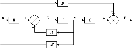
Ki
0
0
0
0
0
0
0
0
0
0
0
⎡0
0
0
0
0
0
0
0
0
0
0
0
⎢⎢ 0
0
Ki
0
0
0
0
0
0
0
0
0
⎢0
0
0
0
0
0
0
0
0
0
0
0
⎢0
0
0
0
Ki
0
0
0
0
0
0
0
⎢0
0
0
0
0
0
0
0
0
0
0
0
(20)
⎢0
0
0
0
0
0
Ki Ф
0
0
0
0
0
⎢0
0
0
0
0
0
0
0
0
0
0
0
⎢0
0
0
0
0
0
0
0
Ki e
0
0
0
⎢0
0
0
0
0
0
0
0
0
0
0
0
⎢0
0
0
0
0
0
0
0
0
0
Ki Ф
0
⎣0
0
0
0
0
0
0
0
0
0
0
0⎦
Integrator works using
Ki
gain.
We multiply the Ki
gain by the difference of the process state and state reference. This multiplication product is integrated and then added by the difference of the previous state followed by multiplication with the gain of K. This process repeatedly occurs throughout the system.
References Translation movement stability control of quad tiltrotor using LQR and LQG
- E. A. Euteneuer and G. Papageorgiou, “UAS insertion into commercial airspace: Europe and US standards perspective,” in IEEE/AIAA 30th Digital Avionics Systems Conference, 2011, p. 5C5-1-5C5-12.
- A. Ashari, A. Dharmawan, D. Lelono, I. Usuman, and T. W. Supardi, “Quadcopter Control System for Natural Disaster Evacuation Support System,” in ICCSE (International Conference on Computer Science, Electronics, and Instrumentation), 2012, pp. 75–80.
- S. Gupte, Paul Infant Teenu Mohandas, and J. M. Conrad, “A survey of quadrotor Unmanned Aerial Vehicles,” in 2012 Proceedings of IEEE Southeastcon, 2012, pp. 1–6.
- L. R. G. Carrillo, A. E. D. López, R. Lozano, and C. Pégard, Quad Rotorcraft Control. London: Springer London, 2013.
- T. K. Priyambodo, A. E. Putra, and A. Dharmawan, “Optimizing control based on ant colony logic for Quadrotor stabilization,” in 2015 IEEE International Conference on Aerospace Electronics and Remote Sensing Technology (ICARES), 2015, vol. 1, pp. 1–4.
- T. K. Priyambodo, A. Dharmawan, and A. E. Putra, “PID self tuning control based on Mamdani fuzzy logic control for quadrotor stabilization,” in AIP Conference Proceedings, 2016, vol. 1705.
- M. Ryll, H. H. Bulthoff, and P. R. Giordano, “Modeling and Control of a Quadrotor UAV with Tilting Propellers,” in 2012 IEEE International Conference on Robotics and Automation, 2012, pp. 4606–4613.
- K. T. Oner, E. Cetinsoy, M. Unel, M. F. Aksit, I. Kandemir, and K. Gulez, “Dynamic Model and Control of a New Quadrotor Unmanned Aerial Vehicle with Tilt-Wing Mechanism,” Int. J. Mech. Aerospace, Ind. Mechatronics Eng., vol. 2, no. 9, pp. 12–17, 2008.
- R. Voyles and G. Jiang, “Hexrotor UAV Platform Enabling Dextrous Interaction with Structures - Preliminary Work,” in IEEE International Symposium on Safety, Security, and Rescue Robotics (SSRR), 2012, vol. 0, no. c, pp. 1–7.
- A. Sanchez, J. Escareño, O. Garcia, and R. Lozano, “Autonomous Hovering of a Noncyclic Tiltrotor UAV : Modeling , Control and Implementation,” in Proceedings of the 17th World Congress The International Federation of Automatic Control, 2008, pp. 803–808.
- M. Ryll, H. H. Bülthoff, and P. R. Giordano, “A novel overactuated quadrotor unmanned aerial vehicle: Modeling, control, and experimental validation,” IEEE Trans. Control Syst. Technol., vol. 23, no. 2, pp. 540–556, Mar. 2015.
- A. B. Chowdhury, A. Kulhare, and G. Raina, “A Generalized Control Method for A Tilt-Rotor UAV Stabilization,” in IEEE International Conference on Cyber Technology in Automation, Control, and Intelligent Systems (CYBER), 2012, pp. 309–314.
- S. Abiko and K. Tashiro, “Fundamental numerical and experimental evaluation of attitude recovery control for a quad tilt rotor UAV against disturbance,” in 2016 16th International Conference on Control, Automation and Systems (ICCAS), 2016, pp. 709–712.
- A. Soukkou, M. C. Belhour, and S. Leulmi, “Review, Design, Optimization and Stability Analysis of Fractional-Order PID Controller,” Int. J. Intell. Syst. Appl., vol. 8, no. 7, pp. 73–96, Jul. 2016.
- A. Nawikavatan, S. Tunyasrirut, and D. Puangdownreong, “Application of Intensified Current Search to Multiobjective PID Controller Optimization,” Int. J. Intell. Syst. Appl., vol. 8, no. 11, pp. 51–60, Nov. 2016.
- A. Nagaty, S. Saeedi, C. Thibault, M. Seto, and H. Li, “Control and Navigation Framework for Quadrotor Helicopters,” J. Intell. Robot. Syst., vol. 70, no. 1–4, pp. 1–12, Oct. 2012.
- A. Dharmawan, A. Ashari, and A. E. Putra, “PID Control Systems Using LQR Approach for Quadrotor Flight Stability,” in International Conference on Science and Technology (ICST), 2016.
- A. Dharmawan and I. F. Arismawan, “Sistem Kendali Penerbangan Quadrotor pada Keadaan Melayang dengan Metode LQR dan Kalman Filter,” IJEIS (Indonesian J. Electron. Instrum. Syst., vol. 7, no. 1, p. 49, Apr. 2017.
- M. H. Amoozgar and A. Chamseddine, “Experimental Test of a Two-Stage Kalman Filter for Actuator Fault Detection and Diagnosis of an Unmanned Quadrotor Helicopter,” J. Intell. Robot. Syst., pp. 107–117, 2013.
- E. Lavretsky and K. A. Wise, Robust and Adaptive Control. London: Springer London, 2013.
- A. Dharmawan, Y. Y. Simanungkalit, and N. Y. Megawati, “Pemodelan Sistem Kendali PID pada Quadcopter dengan Metode Euler Lagrange,” IJEIS - Indones. J. Electron. Instrum. Syst., vol. 4, no. 1, pp. 13–24, 2014.
- A. Dharmawan, A. Ashari, and A. E. Putra, “Mathematical Modelling of Translation and Rotation Movement in Quad Tiltrotor,” Int. J. Adv. Sci. Eng. Inf. Technol., vol. 7, no. 3, p. 1104, Jun. 2017.
- R. W. Prouty, Helicopter Performance, Stability, and Control, 2002nd ed. Krieger Pub Co, 2002.
- K. Ogata, Modern Control Engineering, 5th ed. New Jersey, USA: Prentice-Hall, 2010.
- M. Athans and P. Falb, Optimal Control: An Introduction to the Theory and Its Applications (Dover Books on Engineering). New York, USA: Dover Publications, 2006.
- R. E. Bellman, Dynamic Programming. New Jersey, USA: Dover Publications, 2003.
- B. Messner and D. Tilbury, “Control Tutorials for Matlab and Simulink,” 2011. [Online]. Available: http://ctms.engin.umich.edu/CTMS/index.php?aux=Home.
- D. A. Bini, B. Iannazzo, and B. Meini, Numerical Solution of Algebraic Riccati Equations. Philadelphia, USA: Society for Industrial and Applied Mathematics, 2012.
- N. Arora and J. R. Saini, “Estimation and Approximation Using Neuro-Fuzzy Systems,” Int. J. Intell. Syst. Appl., vol. 8, no. 6, pp. 9–18, Jun. 2016.
- J. F. Shepherd and K. Tumer, “Robust neuro-control for a micro quadrotor,” in Proceedings of the 12th annual conference on Genetic and evolutionary computation - GECCO ’10, 2010, p. 1131.
- E. Pfeifer and F. Kassab Jr., “Dynamic Feedback Controller of an Unmanned Aerial Vehicle,” in 2012 Brazilian Robotics Symposium and Latin American Robotics Symposium, 2012, pp. 261–266.
- C. Di, Q. Geng, Q. Hu, and W. Wu, “High performance L1 adaptive control design for longitudinal dynamics of fixed-wing UAV,” in The 27th Chinese Control and Decision Conference (2015 CCDC), 2015, vol. 1, no. 1, pp. 1514–1519.
