Travelling breaking waves

The theory of surface gravity waves is a classical branch of hydrodynamics [1–4]. However, the modelling of the wave breaking remains a difficult subject [5–7]. We study a recent model of breaking waves proposed in [8, 9]. The equations are derived by using the depth averaging of the equations for mass, momentum and kinetic energy. The model describes the wave breaking phenomenon by introduction of a new variable that is enstrophy (squared vorticity) following the works [10–12]. However, compared to the above mentioned papers, the enstrophy generation is not related to the shock formation, but rather to the turbulent dissipation. The model is mathematically simpler than two-fluid models describing a fine structure of the vorticity formation and propagation developed further in [13] and generalized to the case of stratified fluids in [14].

The model contains two empirical parameters. The first one controls turbulent dissipation. The second one is responsible for the eddy viscosity and is determined by the turbulent Reynolds number. We study travelling waves solutions to this model.

The paper is organized as follows. In Section 2, we present the governing system of ordinary differential equations (ODE) for travelling waves. In Section 3, the Lyapunov function for the corresponding ODE system is derived, and in Section 4 the behavior of the solution to the ODE system is discussed.

1.    Problem Statement

The following system of equations is established in [8]:

∂h дй + dhU

∂t

∂hU

= ° ,

∂x

+ 9 hu2 + gh +   + h2h = 8 / 4 h dx \        2           3 / ox Ree

∂U ϕ∂x

,

8 h, ₊ 8 MJ» = ®^»8MTX ² - с , _hv 3 . ∂t ∂x Re ∂x

Here h is the water depth, U is the depth averaged horizontal velocity, g is the gravity constant and ϕ is the enstrophy variable. The system depends on two parameters: Re that is the Reynolds number and C r that is the turbulence dissipation parameter. In system (1), the first equation is the conservation of mass, the second one is the conservation of momentum, and the third one is the enstrophy equation. The “dot” means the material derivative:

• : dh , _{T T} dh у д⁹ тт⁹\ i. dt + Udx, (dt + U dx) ^.

We are looking for travelling wave solutions to (1). Let us introduce the travelling wave coordinate £ = x — Dt . Here D = const is the wave propagation velocity. The time and space derivatives are transformed as follows:

∂d

∂x ^→ dξ ^, ∂d

-

∂t dξ

From the mass conservation equation we get: h(U — D) = m. Without loss of generality, we can suppose that m > 0, i. e. the flow propagates through the front from left to the right. Then h = (U - D)h, and m2 h′ ′ h =           ■ where h‘ = —. Using these expressions, we reduce the momentum equation to the dξ following form:

mdU ₊ ' ( gh 2 ₊ ,,, ₊ | m 2 (£)) - » ( * h3^ ) = o .

dq dq \ 2          3 h \h J J dq Ree      dq /

It is important to note that system (1) is invariant (i.e. it retains its form) under the Galilean transformation:

x = x + Vt,

U = U + V, t=t with

• V = const .

Therefore, without loss of generality, we can consider the case where the wave speed of travelling waves is D = 0, i.e. the solution is stationary. Integrating once with respect to ξ , we obtain m2 + gh2 + h3^ +  m2 (h)‘ +   h2mV^ () = I = const.

• h 2          3 h \h J Re \ h /

This equality is equivalent to the following equation:

(9 =

3 I    3    3gh 3h^ 12hy^

h

hm ² h ² 2m ²    m ²     Rem

For convenience, we introduce the variable Q by h = e Q . The equation of momentum can be written as follows:

.‘ = ^{3 I}e -Q _ 3 e - 2Q - ³ g _e Q - 3 ^e 2Q - ^{12 P}V^ _e Q m ²              2 m ²     m ²       Rem '

Q ‘ = P.

The equations for enstrophy becomes:

, Sh^ / m, A²   _ , 3

= R Г h2 ^h ) ^- C r ^h * ² '

or

^ϕ Reh h

C r hϕ ³2 m

.

It is easy to show that the above equality is equivalent to

, ^{8mP 2}V^ __Q C r ^ ² _Q

Ф = —-—e ^Q-- e ^Q .

Re        m

Therefore, system (1) can be written as

' Q‘ = P, p‘ = 3Le-Q - 3e-2Q - 3g eQ - 3^e2Q - 12P^^eQ m2            2m3 2    m2      Rem

^ = ^{8 mP 2} y ^ e- Q - C r p₁ e_Q. Re        m

In the case when ^ = 0 , system (2) is Hamiltonian, i.e.,

Q ‘ = P,

P ‘ = ^Ie - Q - 3 e ^-2Q - m ²

^{3 g} _e Q

2 m ²

The Hamiltonian of system (3) is defined by

H (Q,P ) = P 2 2 -

3 e ^- 2Q ₊

J^_eQ 2 m ²

+

3 I m ^{2 e}

Indeed, we can check that dQ ∂H d£ = dP’ dP ∂H d^ = - dQ.

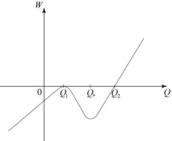
Fig. 1 . The graph of the potential energy W(Q)

Let us present the Hamiltonian as the sum of kinetic and potential energy

H (Q,P ) = P + W ( Q ) ,

where

W ( Q ) = - 3 e ^-2Q + f^Q + ^|e ^-Q .

2      2m ²      m ²

The graph of the potential energy W ( Q ) is shown in Fig. 1. We introduce the critical points Q 1 and Q * of W ( Q ) :

∂W dQ |Q=Q1     ’

and

∂W dQ Iq=q'     .

Without loss of generality, we can assume that W(Q1) = 0 . Indeed, if W(Q1) = W 1 = 0 , we can replace W(Q) by

W ( Q ) =

^^^^^^^^e

3 e ^-2Q + ^^e ^Q + 3(e ^-Q — W i •

2      2m ²      m ²

To justify the behaviour of W ( Q ) shown in Fig. 1, we formulate the properties of W ( Q ) in the following proposition.

Proposition 1. Let Q1 < Q* (or, equivalently, h1 < h*) be the critical points of W(Q). Then | U11 > Vgh1 and |U* | < Vgh* ■ It means that the flow ahead of the front (at h = h1) ∂2W is supercritical and behind the front (at h = h*) is subcritical. Moreover, dQp |q=Qi < 0, ∂2W and dQp ^Q- > 0

Proof. Denote by M1 = (Q1, 0) and M * = (Q * , 0) the singular points of system (4). Then

∂W ∂Q

= 3Ц exp^{( - Q )} fm ² exp^{( - Q )} + g ^exp(2Q⁾ - Л . m2                           2       /

Replacing again exp( Q ) = h , we get that in the critical points

∂W ∂Q . 3 gh^_ m2h \ 2 । m2 -1^ = 0. In particular, this implies gh2 m2 2 + ЛТ = gh* + 2+ m2 h∗ or (h* — h1) (hlh* gh∗ - 2 gh) =0 m2 Then h* > h1 and -—— = h1h∗ gh* + ghl imply that gh∗ > gh* + ghi 2 + 2 m2 h1h m2 > 2, ∗∗ which implies |U∗ | < gh∗ . Finally, the inequality gh∗   gh1    m2    m2

^{gh 1} <  2'2 = м* <% '

implies | U ₁ | > gh ₁ . The inequalities for the second derivatives are direct consequences

of the inequalities because sign proved.

_∂ 2 _W

∂Q ²

| Q=Q i = -^sig^{n( U} i2

— gh i ) , i = 1 , * The proposition is

□

This proposition establishes the behaviour of the function W(Q) shown in Fig. 1.

2.    Lyapunov Function

The Lyapunov function for system (3) is derived from the energy equation. Let us write down the energy equations [8]:

£ + Л Ue + U Лзр + h + h2h — 4VTh^) ) = —h « e > . dt dx у         у 2     3

2        2         * 2

Here e = ——I—^ + "6" + g^ • For travelling wave solutions the energy equation takes the form:

( m ³ ( h ) ml myh ² ghm  m³ \ h

6 V h / + h + 2 +2

where « e ^= -r- h ² y ^3/2 . Therefore, the Lyapunov function for system (3) is

• L(Q,P,^) = m.P 2 + mIe-Q + m^Q + ^gm .

  _-

  
  

  ^m3 -2Q

  2 e •

  
  
3.    Existence of Travelling Wave Solutions

6                   22

The graph of the Lyapunov function is shown in Fig. 2.

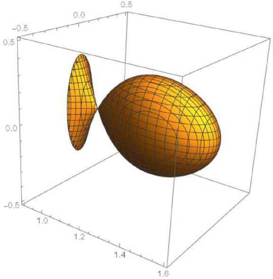
Fig. 2 . The graph of the Lyapunov function

Denote Q : у = Q 2 . Then system (3) takes the form

(Q‘ = P, p‘ = ILe-Q - 3e-2Q — 3g eQ — 2°2e2Q — 12P|Q| eQ

^<     m2             2 m ² m2      mRe

_Q , = ^{4 m}P sgn ^(Q) e — Q - C r QQ e Q

<         Re            2m

As in the case of system (3), there are two singular points with the same properties as in the case of simplified system (3). Denote them by M1(Q1, 0 , 0) and M * ( Q * , 0 , 0) .

Linearisation system (4) gives us only the information on ( Q, P ) , that is we know that locally (Q — Q1, P ) behaves as follows:

(Q — Q1,P) « (a,b)e*, where the eigenvector (a, b) and the eigenvalue A are the same as in the system with Q = 0. Let us find them. Without loss of generality, we consider the case when Q > 0. System (4) has the form

Q , = P,

P ‘ = ^|e -Q — 3 e -2Q — -^e Q — 30 2 e2 Q — 1^ e Q

m 2             2 m 2     m 2      Rem

q, = 4mP_ e — Q — C r Q2 e Q

Re       2 m

We linearize system (5) at the point M1(Q1, 0 , 0) . Then the first two equations are

separated to give the system

(P‘) = a(P).

where

A ^— (- mg e Q + 3 е " 2» 0) .

The characteristic equation of the matrix A is defined by

The eigenvalues are

| A - AE | =

- λ

-  eQi + 3e-2Qi m2

- λ

= 0 .

λ ₁

J - ^ge Q i +3 e ^-2Q i , m ²

and

λ 2

\ge ^{Q 1} + 3e ^{2Q 1} . m ²

Then Proposition 1 implies that

^ge Q i +3 e ^-2Q i >  0 , m ²

therefore A , >  0 and A ₂ <  0 . This corresponds locally to the saddle point: there exist one-dimensional stable and one-dimensional unstable manifolds. The corresponding eigenvectors are

^— - ( A , ) ■ ^— - (У •

Now, let us look for Q in the form: Q ^ we^t, where ^ and w are found as functions of a and b — aA. Obviously, in the leading order, we have from the third equation: w ~ А^2e-Q1 and ^ — 2A. Then we can represent the solution in the form f Q - Q1

aeλ1 ξ, aλ1 eλ1ξ,           as

^{4ma 2 λ 2}1 - Q 1 2λ 1 ξ

Re e e ^,

ξ → -∞ .

P

[q

This asymptotic behaviour means that one enters (when ξ is increasing from -∞ ) at the point M , ( Q , , 0 , 0) into the compact domain shown in Fig. 2 of the surface L — 0 along the unstable manifold which is degenerate ( Q is decreasing much more rapidly compared to P , Q - Q, as £ — -to ). When £ — to , the solution approaches the point M * ( Q * , 0 , 0) as £ — — +^c .

Now consider system (5) at the point M * ( Q * ;0;0) . Perform the linearization at M * ( Q * ; 0; 0) and get the eigenvalues and eigenvectors in the form:

A 2 —

a/ ge Q * + 3 e ^{2 Q}* m ²

A T — a /—ge Q * + 3 e ^{2 Q}* , 1        _m 2

and

-—-  ¹     -—-

V ^{1 —} V1J , V ^{2 —} ^A2j •

Proposition 1 implies that

3^_eQ* ₊ 3 e ^-2Q* m ²

< 0 ,

therefore A i and A 2 are imaginary complex numbers. Since A i ₂ = ik, k E R , the singular point of M * ( Q * ; 0; 0) is a center point considered in the plane of P, Q -variables. However, since L is the Lyapunov function, the solution tends to the state M _∗ , i.e. the fixed point M _⋆ is asymptotically stable. For a fixed value of C _r , the solution behavior in the neighborhood of the point M * (Q * ; 0; 0) depends on the Reynolds number. For large Reynolds numbers, it is oscillatory (the case of low dissipation), for small Reynolds numbers it is monotonic (the case of large dissipation). Now we fix the values C r = 0 , 48 , h i = 1 , m = 4 , g = 9 , 8 . The critical value R = R c и 0 , 71 corresponds to the transition from a monotonic profile to an oscillatory one (see Figs. 3 – 5).

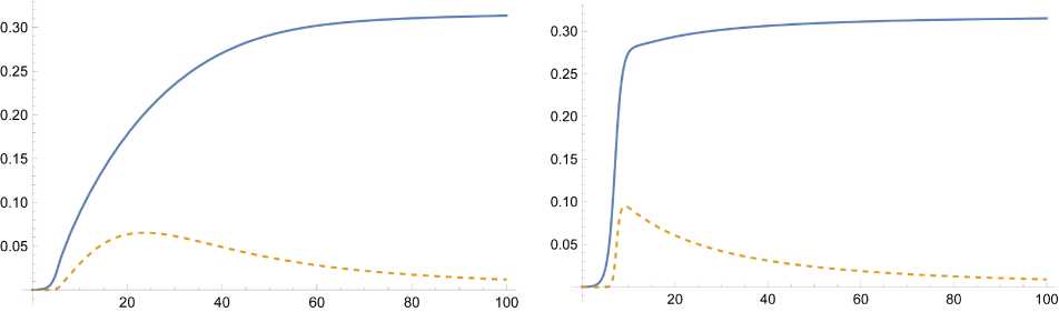
Fig. 4 . R = R c и 0 , 71 and C r = 0 , 48

Fig. 3 . R = 0 , 1 c и 0 , 71 and C r = 0 , 48

20          40          60          80          100

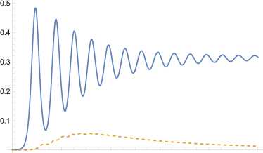
Fig. 5 . R =10 > R c and C r = 0 , 48

Conclusion

In this paper, the problem of modelling breaking waves in shallow water is considered. The existence of an analytical and numerical solution to the problem in the form of a traveling wave is shown. The singular points of the system are described. It is shown that there exists a critical value of the Reylnols number corresponding to the transition from a monotonic profile to an oscillatory one.

Acknowledgments. The author would like to thank Professor Sergey L. Gavrilyuk for posing the problem and attention to the implementation of this work. This research has been funded by the Science Committee of the Ministry of Education and Science of the Republic of Kazakhstan (Grant no. AP09259578).