Tuning stacked auto-encoders for energy consumption prediction: a case study

Published Online February 2019 in MECS DOI: 10.5815/ijitcs.2019.02.01

Each part of a computer needs electrical energy to pursue its duty. A computer system can be divided into two categories: hardware and software. Researchers have long discussed distinctive properties of them in terms of energy consumption (EC) [1,2,3]. A processor is a hardware component that interacts with a large portion of a computer system.

Processors are of great importance in energy consumption rate of a computer system [4]. They are executed in accordance with the commands of an operating system which manages processors. One can assume a computer system as a factory in which a processor can be regarded as a heavy worker of it. Because processors handle with data streams due to mainly input/output operations.

To perform a profiling or prediction on energy consumption data, traditional methods such as random forest [19], naïve Bayes [20], and support vector machine

(svm) [21] are frequently employed. However, such methods may not yield accurate results with real-time long-term data. In order to address this problem, deep learning [22] has emerged as a robust technique. Developments in neural networks have led to the adoption of some types of deep neural networks. Recent advances in hardware components such as GPU may have supported this process.

SAE is a preferable deep learning method due to its advantages over traditional auto-encoders [23]. It provides hierarchical grouping for auto-encoder that ensures robustness in the structure of deep networks. Further, SAE is a robust unsupervised method that enables practitioners to create a large number of hidden units in deep neural network layers.

Despite the fact that deep neural networks have been applied for energy consumption profiling, SAE has not been investigated in terms of processor energy profiling. On the other hand, optimizing various parameters creates a favorable effect on profiling methods by increasing the prediction accuracy. In recent years, deep learning methods have been applied on various fields such as wind power prediction [15], traffic data flow prediction [16], and image processing [8] without considering tuning parameters. Underlying motivation of selecting processors to perform the experiment is that they are easy to be exposed measure energy consumption. In addition to this, processors give tips for analyzing design patterns of programs being executed.

In this work, the effects of tuning parameters of SAEs on processor energy consumption prediction are investigated. To this end, 14 data sets retrieved from the executions on the same processor are exposed to a data processing for deep learning. Thereafter, energy consumption rates are predicted with both tuned and basic SAEs. According to the obtained results, tuning SAEs provides two percent increase in accuracy.

The rest of the paper is organized as follows: Section II summarizes the literature. Notions and background are described in Section III. The experiment and the results are detailed in Section IV. Conclusions are given in Section V.

• II.    Related Works

When the literature is examined in detail, it is clearly seen that SAE has been generally applied for image processing, biomedical detection systems, speech and audio processing, and energy profiling.

Lin et al. [5] proposed a dynamic data-driven approach for stacked auto-encoders. Their method mainly depends on an association rule analysis to determine the weights of input data. A simulation was designed based on weather forecasting data. The method produced promising results for dynamic data environments that it was able to reduce average error rate up to 87%. One of the important application topics of SAEs is traffic flow prediction. Zhou et al. [6] proposed a SAE-based ensemble method that yielded higher accuracy than the alternatives such as ANN, LSBOOST, and SAE. Forecasting any trend requires a sophisticated method to build a reliable model. To this end, SAE could be a feasible solution. In [7], a stacked auto-encoder namely SAEN was developed for tourism demand forecasting. It outperformed some widely known competitive methods such as seasonal autoregressive integrated moving average, and multiple linear regressions.

There has been a great interest in the application of deep learning approach in image processing [8-10]. SAE was also applied on medical image processing. In, a SAE framework was developed for detecting nuclei on breast cancer histopathology images [11]. The method was then compared with nine alternatives. According to the results, SAE framework requires average training time. However, it yields the highest accuracy in almost minimum time compared with the others. Audio processing is another application field of SAE. Deep learning methods have a great potential to be applied on audio data. Such a method was proposed by Luo et al. [12] to detect double compressed audio in codec identification. SAE achieved better results than traditional methods including neural network and deep belief net. Proposed method was found to be very effective with large-scale data sets. The number of decoders and encoders is equal in traditional stacked auto-encoders. However, a recent study [13] presented a stacked auto-encoder having unequal number of encoders and decoders. The method was able to produce promising results for classification and compression problems. SAE is suitable for classification problems. For instance, in plant classification [14], three different auto-encoders were evaluated. The method achieved up to 93% accuracy for classification. Optimizing SAE parameters could create a favorable effect on the learning problem being handled. In [15], a forecasting algorithm was designed using SAE and back propagation. To increase the accuracy of forecasting, particle swarm optimization was adopted. The method was then compared with basic back propagation and support vector machine. The error of the method is stable at increasing forecasting steps. Video processing is an interesting application area of SAE. For collision detection in densely loaded motorways, a SAE framework [16] tested on large videos. The method was able to detect collisions up to 77.5%. However, there are various threats to validate the method in low traffic patterns.

When some deep learning techniques are evaluated together, the size of training samples is crucial. In a comprehensive evaluation of three types of deep learning techniques [17], reducing the number of training instances adversely affect the accuracy. Lv et al. developed a deep learning method to predict traffic flow. They adopted a greedy algorithm to pre-train the deep neural network. The method was found superior to the competing ones such as support vector machine.

Romansky et al.’s work [25] may include more relevant experimental model to ours in literature. They used deep time series to predict mobile software energy consumption. According to their findings, deep neural models are competitive with state-of-the-art models such as SVM.

• III.    Preliminaries

• A.    SAE

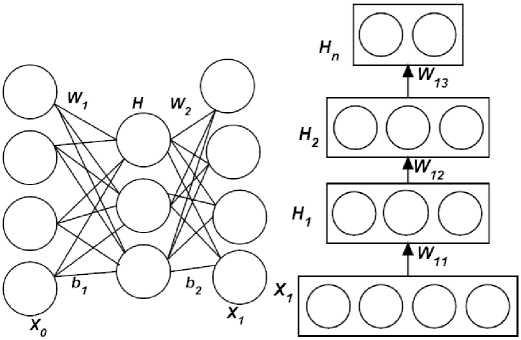
An auto-encoder (AE) consists of a single layer. An output in an AE is used for generating input. An example of an AE is given in Fig. 1-a in which the weight matrix is represented with W and b denotes a bias vector. H and X 1 are the outputs of hidden layer vectors. If input nodes are represented with x 0 …x n, , n is the number of the nodes that are used for generating output y. Fig. 1-b shows a stacked auto-encoder that consists of multiple autoencoders. Each hidden layer output is used as the input of a higher level auto-encoder. Generally, top of SAE is considered as the highest level of auto-encoders. As the level increases, the number of input nodes reduces.

(a)                                   (b)

Fig.1. An illustration of auto-encoder and stacked auto-encoder (a) auto-encoder, (b) stacked auto-encoder

• B.    Energy Consumption Prediction

If some sets of energy data are denoted with e 1 ….e m , m is the number of features. In a processor energy meter, these features could include some metrics such as elapsed time, cpu frequency, and processor power. In order to perform a prediction experiment, e 1 ….e m, is generally divided into two data sets by using percentage split or fold-based cross validation. In this paper, 10 fold cross validation is repeated for 10 times. For each iteration, one part of the data sets is used for testing while nine parts are of testing.

Let y denote the class of a feature set. Since energy consumption rates change greatly in ranges, they should be factored via threshold values. For instance, in a data set, while 0.1-0.5 joules can be represented with 1, 0.6-1 and the other ranges can be represented with 2 and 0, respectively.

Energy consumption data have some metrics such as frequency, graphic frequency, and package power limit which are constant for all the instances. They should be eliminated before training process to obtain reliable prediction results.

• C.    Measuring energy consumption on a computer system

In a traditional way, energy consumption can be calculated via Eq. 1. Here P denotes the power spent in a specific time interval T. By multiplying these parameters, consumed energy can be calculated.

E = P . T (1)

To measure energy consumption, there are various alternatives depending on the device being analyzed. For instance, PETRA [26] is an energy meter that is used for measuring energy consumption of mobile programs. PETRA can be executed via a jar file that makes it easy to use. An address of an .apk is given to the user interface of PETRA by executing Monkey test runner. However, PETRA needs to be updated frequently so that it is very sensitive to the type of operating system.

Jalen [27] is another tool for measuring energy consumption of a program. It can be run via a jar file along with the path of the program to be measured. However, Jalen is for linux operating systems and it does not regard processor in terms of energy consumption.

In this paper, Intel Power Gadget [28,29] is employed for recording energy consumption of processors. It helps users to monitor and estimate processor package power.

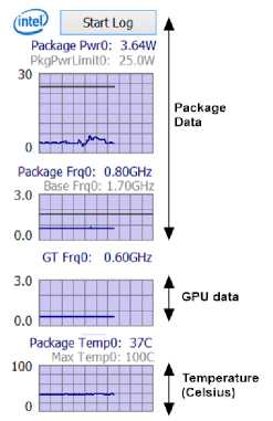
Fig.2. Data monitoring screen of Intel Power Gadget.

Fig. 2 shows main screen of Intel Power Gadget. It provides users detail information including package power, GPU frequency, and temperature. In this screen, user starts monitoring by clicking log button. This operation creates a .csv file in which power consumption details are saved.

• IV.    Method

• A.    Data Sets

To generate energy consumption data sets, 14 software programs have been run in compliance with random 100 test cases. Intel power gadget has been used for recording data sets. It is a user friendly tool that records energy consumption details of processors while executing some processes. Recorded features are as follows: System Time, Read Time Stamp Counter, Elapsed Time (sec),CPU

Frequency_0(MHz), Processor Power_0(Watt), Cumulative Processor Energy_0(Joules), Cumulative Processor Energy_0(mWh), IA Power_0(Watt), Cumulative IA Energy_0(Joules), Cumulative IA Energy_0(mWh), Package Temperature_0(C), Package Hot_0, GT Power_0(Watt), Cumulative GT Energy_0(Joules), Cumulative GT Energy_0(mWh), Package Power Limit_0(Watt), and GT Frequency(MHz). IA denotes package and cores, whereas, GT is the graphic processing unit.

• B.    Data Preprocessing

Input, output, and main steps of the preprocessing operations are given in Algorithm 1. Here EC represents a matrix of energy consumption values.

Algorithm 1 is used for preparing data sets to be exposed to SAE. 1-4 steps are designed for eliminating features having constant values. For instance, GT Frequency (MHz) has been eliminated because it is 600 for all the instances. 5-9 steps are for deleting nonnumeric values of the data sets. In the experiment, IA Power_0 (Watt) feature is determined as prediction class. Step 10 assigns i to 11 that is the number of features after nine steps. Energy consumption values changes between 0-2 for all the test cases so that 11-16 steps make IA Power_0 suitable for prediction by changing its values to 0 or 1 by considering energy consumption rates that enables us to perform receiver operating characteristic analysis.

Input: EC matrix including recorded instances.

As n denotes the number of rows, m represents the number of columns.

Output: New EC matrix _____________________

• l. Fori-N-----1 tom

• 2.    If(isStable(EC,))

• 3.               Delet e(EC,)

• 4.    End For ____________________________________

• 5.    Fori ^----- 1 tom

• 6.    Forj -N------1 ton

• 7.             DeleteNonNumeric(EC₀)

• 8.    EndFor

• 9.    EndFor

• 10.    i <------11 (This column includes

• 11.    Forj ^------1 to n

• 12.     If(EC^

• 13.     ЕСц=0

• 14.     Else

• 15.     EC_S=\

• 16.    EndFor

• 17.    ReturnEC

LAEnergy values to be predicted)

formulated as in Eq. 2 in which possible choices of each parameter are c .

O ( — * C d cos( a * ( 2 ))) m

• 1.    D N------ read csv file

• 3.    control ^— trainControl(method="repeatedcv", number= 10, repeats=3)

• 4.    grid^—expand.grid(layerl=c(80,85,90),

• 5.    parameters ^—train(energy~., data-D_r/, method="dnn", trControl=control, tuneGrid=grid)

l.D^.D^ N----- divide(D)

layei2=c(10,20,25), Iayer3=c(2,3.5). hidden_dropout=3, visible_dropout=3)

The experiment is performed with R package via “caret” and “mxnet” libraries. “caret” is a machine learning library coded with S language of R to perform tuning algorithms. “mxnet” provides practitioners to create deep neural networks for specific purposes. They are easy to learn for practitioners who cope with tuning problems of machine learning algorithms. Algorithm 2 searches best parameters of SAE. First, as in step 1, data is read from a “csv” file. Thereafter, it is divided into training and testing parts (Dt1, Dt2). Step 3 determines control method which is utilized in Step 5 for training via grid search. The bounds of parameter space are in Step 4.

• 1.    model N-----mx.mlp(Du, parameters.

• 2.    preds 4----- predict(model, D^

• 3.    control 4— trainControl(method- 'repeatedcv". number=10, repeats=10)

• 4.    pred.labelN— max.col(t(preds))-l

• 5. tabletpred-labeTD^)

eva 1. met ric=mx. metric. accuracy)

Algorithm 3 predicts energy consumption rates by using detected parameters of SAE. Parameters are produced by Algorithm 2. “mx.mlp” function generates SAEs to build model. Step 2 predicts energy consumption rates based on optimized SAE model. Energy consumption prediction is a multi-class problem so that softmax function is used in the model for assign probability to each class. Eq. 3 calculates softmax function. Here f(x) denotes softmax function and x is an input vector. K is the number of output units and i enumerates output units.

C. Tuning Parameters of SAE

Grid search algorithm is used with manual grid in the experiment. It is a simple tuning strategy that searches a given list of hyperparameters. Grid search selects the best parameters from search space by comparing performance parameters. If total number of predictions is denoted with P in the dimension d, the complexity for m steps can be

f ( x ) _i

_ex i

K

Z e

j = 1

Table 1. Formulas of performance parameters.

Name	Formula
TPR	TP/(TP+FN)
FPR	FP/(FP+TN)
accuracy	(TP+TN)/(TP+TN+FP+FN)
RMSE	1 Г 1                 212 - Z ( yi - zi ) L L ' - 1              J

• D.    Performance Parameters

Three performance indexes are used in the experiment to evaluate the effectiveness of tuning. They are rootmean square error (RMSE), accuracy, and area under the curve (AUC) which is obtained drawing true positive rate (TPR) against false positive rate (FPR). The formulas of the performance measures are given in Table 1. For RMSE, y i is the observed energy consumption, and z i is the predicted energy consumption. n is the number of observations. Other formulas are generated from the notions of confusion matrix.

• E.    Results

  Mean accuracy values of the experiment are presented in Table 2. Tuned and basic SAEs are compared with 20 epochs. According to the obtained findings, in the second iteration, tuned SAE was able to achieve the best accuracy with 0.742857. On the other hand, the best accuracy of SAE is 0.542857. Further, in basic SAE, as the number of iterations increases, accuracy declines inconsistently that for some iterations, accuracy increases. Using tuning operation on SAE improved accuracy up to 0.2.

Table 2. Mean accuracy values of 100 test cases. Bold-faced values are the best for each column.

Iteration number	Tuned SAE	Basic SAE with random parameters
1	0.67619	0.542857
2	0.742857	0.533333
3	0.742857	0.552381
4	0.742857	0.552381
5	0.742857	0.485714
6	0.742857	0.485714
7	0.742857	0.466667
8	0.742857	0.485714
9	0.742857	0.495238
10	0.742857	0.495238
11	0.742857	0.47619
12	0.742857	0.466667
13	0.742857	0.47619
14	0.742857	0.438095
15	0.742857	0.438095
16	0.742857	0.47619
17	0.742857	0.466667
18	0.742857	0.47619
19	0.742857	0.438095
20	0.742857	0.438095

Table 3. Mean RMSE results for tuned SAE. Bold-faced value is the best.

layer1	layer2	layer3	RMSE	Rsquared
80	10	2	0.51488	0.16805
80	10	3	0.528638	0.141662
80	10	5	0.511084	0.144412
80	20	2	0.518676	0.189492
80	20	3	0.521836	0.175013
80	20	5	0.522578	0.156506
80	25	2	0.507903	0.149588
80	25	3	0.532979	0.175687
80	25	5	0.501979	0.184426
85	10	2	0.507076	0.164327
85	10	3	0.506222	0.17498
85	10	5	0.516843	0.1605
85	20	2	0.520204	0.128154
85	20	3	0.509162	0.148409
85	20	5	0.519032	0.158413
85	25	2	0.52041	0.117148
85	25	3	0.533475	0.154795
85	25	5	0.522118	0.159829
90	10	2	0.513195	0.180583
90	10	3	0.519889	0.151531
90	10	5	0.522863	0.161013
90	20	2	0.517321	0.182455
90	20	3	0.532141	0.141483
90	20	5	0.515681	0.14772
90	25	2	0.507656	0.137887
90	25	3	0.528421	0.171819
90	25	5	0.513364	0.122673

Table 3 shows average grid search results of the test cases in terms of tuned SAE. Best configurations are determined by searching optimal number of hidden layers in layer1, layer2, and layer3. According to the experimental results, (85, 25, 5) is the optimal. Compared to the basic SAE, tuned SAE reduced RMSE up to 0.5 that basic SAE was able to achieve 0.57 RMSE with random parameters.

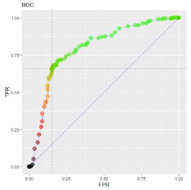
Fig.3. ROC curve of SAE generated using random instances without tuning.

Fig. 3-4 illustrate AUC values of basic and tuned SAE, respectively. Basic SAE achieved 0.79 value of AUC, whereas tuned SAE outperformed it with 0.84 value of AUC. Selected test cases may have affected this difference. However, RMSE results support the evidence provided by values of AUC. Using merely energy consumption data retrieved from processor could create a threat to the validity. However, performing a preprocessing on EC data as in this paper helps removing that threat.

• F.    Threats to the Validity

Executing test cases having similar coding structure could create an internal threat. To alleviate this threat, a random selection has been made on the test case pool.

Using same parameter settings for comparing tuned SAE with basic SAE could create misleading results. We changed parameter settings randomly in basic SAE to create a reliable comparison setting.

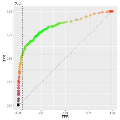
Fig.4. ROC curve of SAE generated via tuning based on grid search.

Algorithm 1 is suitable for imperfect data instances so that it was compared with three alternatives including Expectation-Maximization (EM) [30], Multiple Imputation (MI) [31], and K-nearest Neighbor Imputation (kNNI) [32]. Complexities of those methods are presented in Table 4. For EM, m is the iteration and n denotes the number of parameters. While k denoted the number of steps in MI, l is the number of versions of the data set. For kNNI, n represents the number of instances and d is the number of dimensions. Even in worst case, Algorithm 1 shows competitive complexity compared with EM and kNNI. On the other hand, MI yields lower complexity than Algorithm 1 in some cases.

Table 4. Complexity comparison of similar algorithms.

Method	Complexity
EM	O (m.n^3)
MI	O (kl+l)
kNNI	O (nd)
Proposed method (Algorithm 1)	O (m.n)

• V. Conclusions

This study focuses on tuning SAEs to improve prediction performance of energy consumption of processors. In this respect, a data preprocessing algorithm is proposed to make data suitable for prediction. To evaluate the findings, tuned SAE has been compared with basic SAE. According to the study results, selecting random parameters to execute a SAE based model does not perform well in terms of prediction accuracy and RMSE. Instead, using parameter search methods such as grid search increases prediction performance remarkably. However, as in [24], developing sophisticated tuning methods may provide new insights into energy consumption prediction.

SAEs have been applied in various fields in recent years. Generally speaking, almost all the studies including a SAE based method for predicting real-time data streams use same evaluation metrics. Developing problem-oriented metrics for SAE may deepen our knowledge to find suitable solution.