Unveiling Autism: Machine Learning-based Autism Spectrum Disorder Detection through MRI Analysis

Discussion, exchanges, and learning abilities are impacted by autism spectrum disorder, a neurodevelopmental disease. Autistic symptoms often emerge in the first two years of life and progress throughout time; however, the disorder can be diagnosed at any age [1]. A wide range of difficulties, including those related to focus, learning, motor skills, sensory processing, anxiety, depression, and other mental health issues, are experienced by those with autism. The current global autism epidemic is massive and growing at a dizzying pace. About one in one hundred sixty children has autism spectrum disorder (ASD), according to the World Health Organization (WHO). While some people with this illness are able to live on their own, others need constant assistance.

The time and money needed to diagnose autism are substantial. Early diagnosis of autism can greatly benefit patients by allowing for the early prescription of appropriate medication. In addition to lowering the long-term expenses connected with delayed diagnosis, it can stop the patient's condition from getting worse [2]. Therefore, there is an urgent need for a screening test tool that can accurately predict autistic symptoms in individuals and determine if they need a thorough autism examination. The test should be easy to use, take little time, and be accurate. Because there is no pathophysiological marker, psychological factors alone are insufficient for the diagnosis of ASD due to the lack of a pathophysiological marker. Psychological instruments can help during the initial assessment by revealing patterns of behavior and degrees of social engagement. Behavioral examinations incorporate a range of tools and surveys to help doctors pinpoint the specific kind of developmental delay in a kid. These include medical history, clinical observations, testing for growth and intellect, and directions for making an autism diagnosis.

A number of recent studies have used structural and functional neuroimaging data to investigate the diagnosis of ASD. Morphological neuroimaging is a vital method for investigating ASD-related brain abnormalities. Magnetic resonance imaging (MRI) methods are the main instruments used to study the brain's structure. Diffusion tensor imaging, magnetic resonance imaging (DTI-MR), and structural MRI (sMRI) images are used to study brain anatomy and anatomical connections, respectively. Functional neuroimaging can also be utilized to examine ASD by investigating the activity and functional connectivity of brain regions [3]. Compared to structural methodologies, brain operational diagnostic tools have been around longer for researching ASD.

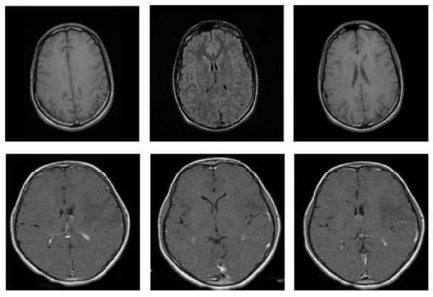
Fig.1. Sample MRI image dataset

Electroencephalography (EEG) accounts for the electrical activity of the brain through the scalp with a high temporal resolution (in milliseconds), and it is the most fundamental method of functional neuroimaging. Researchers have shown success in diagnosing ASD using EEG data. Among the many imaging modalities being explored for functional brain diseases, functional magnetic resonance imaging (fMRI)—whether in a resting-state or task-based configuration—has shown great promise. The spatial resolution of fMRI-based approaches is very high (millimeters), but the temporal resolution is limited owing to the brain's hemodynamic system's delayed response and the time limits of fMRI imaging. As a result, these techniques are not appropriate for recording the quick dynamics of brain processes. Furthermore, motion artifacts are easily picked up by these methods. A sample MRI image dataset is shown in Fig 1.

It is important to note that the third, less common modalities of electrocorticography (ECoG), a form of functional near-infrared spectroscopy (fNIRS), and magnetoencephalography (MEG) can also achieve acceptable performance in ASD diagnosis, according to research. The best way to help doctors correctly diagnose ASD is to use machine learning methods in conjunction with anatomical and functional data. There are two main types of machine learning approaches used in autism spectrum disorder (ASD) research: conventional methods and DL methods. There has been far less effort to investigate ASD or develop rehabilitative solutions using DL techniques compared to more conventional approaches.

Autism Spectrum Disorder (ASD) affects approximately 1 in 36 children, making it a significant public health concern. Early diagnosis is crucial for effective intervention, yet current diagnostic tools often rely on subjective observations, which can lead to delayed or inconsistent diagnoses. Magnetic Resonance Imaging (MRI)-based diagnostics has the potential to revolutionize this process by providing objective and reproducible insights into brain structure and function. MRI offers a non-invasive and detailed view of the brain, capable of capturing the subtle structural and functional anomalies associated with autism. These characteristics make MRI an ideal candidate for machine learning applications aimed at enhancing diagnostic accuracy and reliability. However, the high-dimensional and complex nature of MRI data presents a challenge for traditional analysis techniques. Machine learning algorithms, on the other hand, excel at identifying patterns and correlations in such data, enabling the development of predictive models that could significantly aid in the early and precise diagnosis of ASD. Despite promising advances, current MRI-based machine learning models often exhibit limited generalizability or focus on narrow datasets. This study aims to address this gap by leveraging advanced algorithms and diverse datasets to develop robust and clinically viable diagnostic tools.

The key contributions of the research article are as follows:

• •    To provide a model for autism prediction that makes use of ML methods and can accurately predict autistic symptoms in individuals of any age.

• •    Using a 2D multislice image preprocessing step, quantify local-regional alterations in different parts of the brain and find the correlations in Curvelet space that reflect abnormal brain folding.

• •    To improve identification accuracy for ASD detection using feature selection and weighting algorithms.

• •    To apply the curvelet transform to areas with a generalized Gaussian distribution, it helps to lower the dimensionality of the features.

2.    Related Works

Here, we review some of the approaches taken too far for the categorization of neurodevelopmental disorders, with an emphasis on ASD diagnosis. The eventual assessment might be impacted by improper pre-processing of neuroimaging data due to its rather complex nature, particularly functional information. Ordinary applications often perform a number of stages in the preprocessing of this information [4]. In fact, pre-processed data is often obtained by applying workflows to datasets in order to facilitate future studies. Typically, a predetermined number of steps are applied to the data during low-level pre-processing of fMRI pictures. To minimize execution time and improve accuracy, prepared toolboxes are typically employed. A few of these trustworthy toolboxes include the following: SPM, FreeSurfer, BET, as well as FMRIB software collections (FSL). Identification of the brain, regional contouring, longitudinal screening, adjustment for movement and slice execution, standardization of magnitude, and translation to an existing template are all crucial and essential parts of fMRI preprocessing.

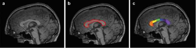
Fig.2. Brain segmentation sample

Brain imaging aims to preserve brain tissue while removing the skull and cerebellum from fMRI images. Territorial flattening takes the signal from neighboring voxels and averages it. Because nearby brain voxels are typically functionally and anatomically connected, this procedure is convincing. Through spatial screening, we can remove noise from polygonal sequences without affecting the signal we're interested in. It is common for participants to shift their heads while undergoing fMRI testing. To ensure that all functional magnetic resonance imaging (fMRI) volumetric pictures have the same voxel dimensions and introductions, mobility adjustment must first synchronize all images to a baseline image.

A common reference time for all the pixels in each fMRI volume image may be achieved by adjusting the time series of the voxels. This is achieved by varying the slice time. The standard practice is to use the reference time that corresponds to the first slice recorded in each fMRI volume picture. To normalize the average intensity of fMRI signals and account for global variances within and across monitoring discussions, this step is called brightness standardization. With General Alpha authorization, studying the human brain, which has numerous cortical and subcortical regions with diverse architecture and functions, is an arduous and complicated process. To get around this, we use brain atlases to divide up brain pictures into a limited number of ROIs, and then we can extract the mean time series from each of those ROIs. Automated Anatomical Labeling is just one of several atlases used by ABIDE datasets, which also provide a wealth of other information [5].

Research into semantic category depiction, word significance, acquiring knowledge, and other related topics has been made possible by the combination of machine learning and deep learning with data from brain imaging [6]. Unfortunately, the complexity of the problem means that machine learning algorithms are still not widely used to diagnose neurodevelopmental disorders, anxiety, and depression, as well as mental health issues like schizophrenia.

In order to identify cases of major depressive disorder (MDD), Craddock et al. employed multivoxel pattern analysis [7]. Twenty healthy controls and twenty people with MDD were included in the forty participants who were analyzed using magnetic resonance imaging (MRI). A 95% success rate was attained by their suggested system. In order to distinguish between individuals with ASD and those without using functional magnetic resonance imaging (fMRI) data, just et al. established a method based on Gaussian Naïve Bayes (GNB) classifiers. In a group of 34 people (17 healthy controls and 17 autistic people), they were 97 percent accurate in identifying autism [8].

Sabuncu et al. performed an encouraging study that employed structural MRI (s-MRI) data and the Multivariate Pattern Analysis (MVPA) algorithm to forecast a cascade of neurodevelopmental illnesses, including mental illness, autism, and dementia. They examined functional neuroscience data from 2800 patients across six websites that are publicly available [9]. The three types of classifiers that make up the MVPA method are Neural Network Approximated Forest (NAF), Retrieval Vector Machinery (RVM), and Support Vector Machine (SVM). Using a 5-fold validation technique, they achieved identification precision of 70% for psychosis, 86% for dementia, and 59% for autism [8].

Research in the fields of clinical neurology, neuroimaging, and deep learning (abbreviated as DNN) has enormous promise. For the purpose of automating the diagnosis of schizophrenia, Plis et al. employed deep belief networks (DBNs) [9]. Applying T1-weighted structural magnetic resonance (sMRI) imaging data, Plis et al. trained a model with three hidden layers. The first layer included 50–100 hidden neurons, while the second and top levels had the same number of neurons. With 198 patients with mental disorders and 191 control subjects, they attained a precision for classification of 90% by analyzing datasets from four separate studies carried out [10].

When it comes to learning concepts from neuroimaging data, DNN defeats traditional supervised learning approaches, such as Support Vector Machine (SVM) 122, as demonstrated by Koyamada et al. Emotional reaction, wagering, linguistic, motor, experiential, interpersonal, and working memory are the seven types of tasks that Koyamada et al. used to characterize task-based functional magnetic resonance imaging (fMRI) data. A median precision of 50.47 percent was attained after training a two-hidden-layer deep neural network [11].

Using transfer learning from two auto-encoders, Heinsfeldl et al. trained a neural network in another study. In addition to allowing neural networks to apply acquired neuron weights in diverse contexts, the transfer learning approach permits alternative distributions to be utilized during training and testing [12]. Heinsfeldl et al. set out to identify ASD and healthy controls in their investigation. One of the primary goals of auto-encoders is to enhance a model's generalizability through unsupervised data learning. Using rs-fMRI (resting state-fMRI) image data from the ABIDE-I dataset, Heinsfeldl et al. performed unsupervised pretraining on these two autoencoders [13]. We translated the knowledge from these two auto-encoders to multilayer perceptrons (MLP) in the form of weights. The accuracy of categorization was up to 70%.

Recently, Mazumdar et al. put forth a novel method for detecting autism spectrum disorder (ASD) in children at an early age by capitalizing on their visual performance while they process visual stimuli, such as pictures. They used an eye tracking device to conduct psycho-visual research. To identify children with autism spectrum disorder (ASD), we merge data from psycho-visual studies with picture attributes and run them through a machine learning system [14]. In order to identify ASD in three open-source datasets from the UCI database, Erkan and Thanh employed various machine learning techniques, including KNN, RF, and SVM. They pooled variables from three separate datasets: "Autism Screening Adult Data Set," "Autistic Spectrum Disorder Evaluation Dataset for Children," and "Autistic Spectrum Disorder Evaluation Data for Teenagers Data Set." It has been demonstrated that the method described in this article may attain a flawless classification score [15].

Observing social interactions is another method for detecting autism spectrum disorder (ASD) using ML. Xue et al. make an attempt in this direction. An analysis method for children's interactions with the NAO robot has been proposed. A system detects autism spectrum disorder in youngsters based on the connection between the content of an image book displayed by a NAO robot and the topic of discussion. To address the problem of data distribution being impacted by inter-site heterogeneity, Wang et al. put out a method [16]. An approach to multi-site domain adaptation based on low-rank representation decomposition has been suggested by the authors.

By computing a common low-rank representation, the suggested solutions lessen the disparity in the distribution of data across several sites. Out of the four sites, one is designated as the target domain and the others as the source domains. This paves the way for the use of low-rank representations to standardize data [17]. In order to discover the best parameters for optimum low-rank representation, machine learning methods like KNN and SVM are employed. They have demonstrated their findings using the (ABIDE) dataset as a case study. ABIDE is a web-based collaboration that shares phenotypic information with control participants and imaging data on individuals with ASD. Eleven hundred and twelve participants from seventeen different countries make up the ABIDE dataset. Classification of autistic subjects from control subjects is accomplished using machine learning methods, specifically KNN and SVM [18]. Wang et al. suggest an additional approach to address the problem of heterogeneity in data obtained from various places. This article presents a strategy for autism spectrum disorder (ASD) identification based on fMRI data that makes use of the Multi-Site Clustering and Nested Feature Extraction (MC-NFE) approach. The suggested approach uses a similarity-driven multiview linear reconstruction method to simulate inter-site heterogeneity. To demonstrate the method's resilience, the ABIDE dataset is utilized [19].

Notably, research has shown that classification accuracy typically declines when using machine learning in conjunction with brain imaging data acquired from many locations, such as ABIDE, to detect autism [20]. We found a similar pattern in this research as well. In their analysis of the ABIDE dataset, Nielsen et al. reached a similar conclusion: locations with prolonged BOLD imaging times had substantially better classification accuracy. On the other hand, fMRI makes use of a technique called blood oxygen level dependent (BOLD) imaging to identify active areas by monitoring changes in blood flow. It would suggest that blood concentration is more active in particular areas compared to others.

Research in this area has centered on studies that employed neuroimaging techniques, including magnetic resonance imaging (MRI) and functional magnetic resonance imaging (fMRI), to identify various neurodevelopmental diseases. Not enough attention is given to the many brain areas that are involved in the prediction of mental diseases [21]. Evidence suggests that certain brain areas emphasize small differences between healthy people and those with neurodevelopmental disorders. Results from a quantitative study utilizing the ABIDE dataset showed that those with ASD had smaller corpus callosums and larger brain volumes. When it comes to moderating actions and processing information, the corpus callosum plays a pivotal role [22]. The biggest connection between the two halves of the brain, the corpus callosum, is made up of over 200 million fibers with different sizes.

Even though the corpus callosum sub-regions did not change significantly between the control and ASD groups, Hiess et al. did find that the ASD group had more volume inside the brain. One method for estimating the size of the brain and its various areas through volumetric measurement is the intracranial volume (ICV). Both Waiter et al. and Chung et al. discovered smaller splenia, genus, and corpus callosum rostrums in individuals with ASD, and both groups also noted smaller isthmuses [23].

3.    Proposed Methodology

This section discusses the various stages of the proposed system to detect autism spectrum disorder based on brain MRI images. These stages include the pre-processing of images, feature extraction, statistical analysis, and prediction model design.

• 3.1.    Pre-processing

This method of characterization is based on the premise that variations in brain activity at different scales should be detectable. The overarching goal of pre-processing is to standardize image magnitudes, eliminate the skull, and divide each instance into a collection of brain areas. The second step is to arrange the volume slices such that they form a 2D picture for each segmented region (the volume). We use the Curvelet transform to examine this 2D picture with the set of slices, and we use a generalized Gaussian distribution to approximately determine the coefficient probability per Curvelet sub-band. As a result, three parameters end up representing each sub-band. Lastly, a traditional support vector machine (SVM) identifies areas associated with autism spectrum disorder (ASD) by performing a binary classification per region. This allows us to assess the generated multiscale descriptor's capacity to discriminate between the two classes.

A mathematical technique for multi-resolution analysis, the curvelet transform works especially well for describing edges and singularities in pictures. For MRI data, where it is essential to capture intricate details and structures, it works well.

The Curvelet transform is particularly good at catching curved edges and tiny details, much like a brush that paints delicate outlines in an image. In contrast, the Fourier transform records frequency information, and the wavelet transform concentrates on localized time-frequency properties. The Curvelet transform is applied in this study to improve the identification of subtle structural characteristics in MRI images that are frequently suggestive of autism. The extended Gaussian distribution is a versatile statistical model that may be used to explain a variety of data types found in MRI scans. It includes both Gaussian and Laplace distributions. In order to properly describe the heterogeneity in MRI data and enable our machine learning model to distinguish between those with ASD and those without, we employ the extended Gaussian distribution. Consider the generalized Gaussian distribution as a curve that changes shape in response to patterns in the data, moving from the bell-shaped Gaussian to distributions that are flatter or sharper.

The goal of pre-processing is to improve the appearance of the baseline image and to make quantitative evaluation more accurate and consistent by applying a sequence of transformations to the image. Nevertheless, depending on the circumstances, there is no pre-defined analytical framework for pre-processing brain MRI. Based on their critical role in enabling electromagnetic radiation assessment and precise numerical contrast throughout multi-modal MRI quantities, the present study utilized co-registration, replication, skull removal, and magnitude adjustment as the starting points for the pre-processing process pipeline.

Even when using the same procedure, cells, cautiousness, and detector, image quantitative analysis becomes more challenging due to variations in the distribution of brain MRI intensity caused by differences in inter- and intra-scanner susceptibility and collection characteristics. To enable radiomics analysis and precise statistical evaluation among MRI magnitudes, sensitivity standardization is necessary to provide a consistent tissue brightness measurement in brain MR images throughout all investigations.

^{h s} =^ s ^{I h} ’^J(^r)^dr (1)

In the above equation, h_s and h j represents the intensity level values of the baseline image and actual image respectively. Upper and lower baseline images are represented as J_s and I_s respectively. In addition to correcting intensity non-uniformity and Gaussian noise, image pre-processing can address additional significant aberrations that are intrinsic to MRI capture. A low-frequency signal on an MRI scan can be caused by intensity non-uniformity, intensity inhomogeneity, or bias in the magnetic field, among other things, including fluctuations in the field itself. Multiple components of the brain's MRI consumption, including gray matter, white matter, and cerebral-spinal fluid, may show varying intensities due to this artifact. The picture shows fluctuations in intensity at high frequencies, which are known as noises. In order to improve the signal-to-noise ratio (SNR) without losing the high-spatial-frequency details of the original image, noise reduction is often used.

The ITK filter was used for skull stripping, while the SRI atlas was used to specify the reference atlas and its related comparative brain masking. In order to align the magnitude levels of the individuals under study with the reference picture of a high-quality modality, the ITK histogram matching filter was used. Regarding noise filtration, the low-level image processing is accomplished by smallest unvalued segment assimilating nucleus was employed. The following is a presentation of the basic rule that governs SUSAN noise filters; this method merely averages the ratios of adjacent pixels in sections of homogeneous brightness.

The first step in fixing brightness dissimilarity simply to fix the fact that intensities were not consistent. This MR bias correction approach uses the subsequent equation as its model of image composition.

D(y) = Ку)С(у) + g(y)

where, D represents the original image with noise, J defines the image without noise C represents variational bias specified in the image and g defines gaussian noise. The resulting image can be represented as D = J + C which is estimated by applying logarithmic function on both the sides of the equation.

Original Image

Co-registration

Resampling

Skull stripping

Normalization

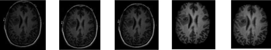
Fig.3. Pre-processing stages of a brain MRI

The brain image that was undergone various pre-processing stages such as co-registration, resampling, skull stripping and normalization are shown in Fig 3.

For the Curvelet characterization, the resulting mosaic must be zero-padded so it fits into a squared form. This visualization may depict morphological alterations such as abnormal cerebral bending despite compromising the crucial image data; it preserves the primary geometric connections of an area in the Curvelet field. Covering region, depth, and folding are not necessarily connected to characteristics in this dimension given this perspective since the object fundamental relationships in the Curvelet dimension cannot possess the normal geometric significance in the context of Euclidean geometry.

While such metrics indicate discrepancies in previous research, the method here aims to capture more nuanced anatomical modifications, such as a loss of global form, that are difficult to discern in terms of size or density. Keep in mind that the amount of original information preserved by each 2D multislice image varies depending on the total number of layers contained in the brain area under investigation, the scanner's image quality, and the specific region under study. Because of its proven ability to approximate complicated geometrical features and textures, the 2D multislice picture is transformed to a curvelet space in order to conduct the multiscale analysis. In addition to the succinct illustration of curvy parametric frameworks, the multiscale geometrical mapping known as the curvelet conversion maintains the same excellent decomposition benefits as the wavelet transform. It is well known that curvelet functions provide sparse illustrations for smoother surfaces that have singularities between curvatures.

Because the number of orientations and the number of micro-locations are directly correlated to the inversion of the scale, which is an additional connection that the anisotropic feature increases, We primarily chose this representation because of its anisotropic curve definition; our goal is to convey aberrations of local and regional forms. Also, certain surface designs, which are meant to depict tissular configurations that connect with neuropathology, can be characterized by the correlation of the quantity of micro-locations with their size.

• 3.2.    Feature Extraction

The characteristics in radiomics may be grouped into four types: first-order, form, texture, and image filtering. In this study, texture characteristics such as GLCM, GLRLM, GLSZM, NGTDM, and GLDM were used. The following image filtering classes were used: wavelet alteration, rectangular, squares shape, Laplacian of Gaussian (LoG), and local binary pattern (LBP). Both the unfiltered and filtered versions of the image were used to extract first-order and textural characteristics. In order to determine the morphology of the ROI (region of interest), only the original pictures were used to extract shape characteristics. The wavelet transforms, a potent instrument for multiscale pattern capture, uses this either systematically describe images according to size (s) and brightness (b).

w⁽t,d) = 1=^ ^ (^) f(u)du (3)

It is able to successfully retrieve details from confined high-frequency transmissions because it examines occurrences with high spatial frequencies that are spatially limited. Using the initial quantities, a high pass or low pass filter was applied to compute the wavelet transformation at each of the eight stages of deconstruction. Two stages make up the Laplacian of Gaussian (LG) filter: first, a Gaussian filter is used to smudge the image. Then, the Laplacian is applied to locate edges, which are locations where the gray level changes rapidly. The following is how the calculation is done. p is the size of the Gaussian filter's core and (c, d) are the geographical dimensions of an image component. The LG filter was used in this research with two different kernel size parameters (p = 1 and 2 mm).

c2+d2

“(с.^- прф -^-Р ’^ (4)

Lambda adjusters are quadratic and root-based image filters. One way to achieve a square filter is by squaring the image magnitudes (I), as shown in the following equation. Another way is to use the squared root of the mean of the intensities (B), as shown in the adhering to equation. After applying these filters, the results are adjusted to fit the initial picture magnitude spectrum.

L ² = (.     ^{, m}      )

m     Jmaxlmum\,m\

/m"^

maximum] Im\Im

■ Jmaximum \Im\Im

! m >0

I m <0

By assigning a probabilistic number to each pixel in the image and then using the center pixel value to limit the surrounding pixels, Regional Probabilistic Pattern (RPP) is able to extract the texture features from the distribution of these labels. In the following equation, where Q is the neighboring pixel samples in the circumference of the neighborhood of the radius s, and corresponds to the size of the histogram, produces numerous binary structures, may be used to describe LBP. The equation (8) gives the definition of g(j_q - j o ), where j_q is the intensity of the surrounding pixel and j_o is the brightness of the center pixel.

RPP(Q,s) = x q:¹o g(j q -j_d)2 ^q                                  (7)

1 gu^h

^{g(j q   J d )}   {0  g(j q )>j_d                                      ⁽⁸⁾

The radiometric types of features were used in this investigation. A simplified and repeatable framework for the characteristics of radiomics extracting procedure was implemented using an open-source Python tool.

• 3.3.    Statistical Analysis

To measure the consistency and repeatability of the radiomics characteristics, this study used the changing fluctuate (CF), together with the most popular indices for evaluating convergence of perpetual parameters in uniformity investigations, the harmony coefficient of determination (HCD) and the intraclass relationship value (IRV). When evaluating agreement, the Pearson correlation coefficient is not the right tool to use because it is more commonly employed to evaluate the linear correlation between sets of quantitative data. The two notions of relationships, concordance and association, are distinct. While consensus looked at whether different processes, assessors, or techniques produced identical results of the computed responses, a significant relationship among two variables does not demonstrate which such two followers can generate the same results because relationship does not reveal systematic variance among viewers.

In this study, the outcomes of the benchmark and adjusted pre-processed images were used to generate the HCD, which was then used to evaluate the agreement across ratters using equation 9, where λ is the mean value as well as δ is the standard deviation. The results were presented with 95% confidence ranges.

HCD(c,n) = 1-

(^ c ~^ n )²+^ c ⁺^ n ~2^a c ^a n

(l_c-l n ) ^c « 2 « n

Overall intraclass relationship value (IRV), which assesses the degree of concordance and consistency between respondents, is provided by Eq. (12) and is a suitable metric for evaluating inter-rater reliability.

IRV(c,n)

S² c

S C +S f

While the IRV and HCD may seem similar at first glance, there are two key differences between the two. Firstly, the IRV is defined for either fixed or arbitrarily participants while the HCD is typically suggested for fixed observers. Secondly, while the HCD is evaluated independently of the ANOVA model, the IRV indexes are necessary for the ANOVA assumption. This means that different versions of the IRVs can produce various outcomes regardless of what is selected ANOVA models. Another factor that might affect the characteristics' stability and reliability is the whole physiological range of values that are seen across patients. Reliability and informative radiomic qualities are determined by the physiological parameters, which are explained by the fluctuating spectrum (FS). Equation 11 is used to determine the FS for both the baseline and modified sample populations, where c is the baseline category, an is the changed disposal, b is the patient count, and к is the case index for the j^th characteristic.

FS(c,k) = 1

—

1 у           lc(k)j-n(k)jl b    ^=1 Ma(r(c,n)j)-Mi(r(c,n)j)

Elements with FS values nearer to one are more likely to be resilient characteristics versus interference and store relatively accurate data. FS scores can vary from 0 to 1. Radiomic characteristics were deemed robust and repeatable in this study if their HCD and FS were greater than 0.85. On the other hand, IRVs with 92% confidence intervals, greater than 0.9, and 0.62-0.89 considered deemed outstanding and satisfactory, accordingly, in terms of reproducibility.

• 3.4.    Prediction Model Design

The original method for autistic characteristic prediction was the Random Forest based autistic Prediction System (RF-APS). The decision tree based autism prediction system (DT-APS) was used for further refinement, and it yielded superior results. Below, we will go over these algorithms in sequential order that were utilized to create the system: When first starting to build the prediction model, the DT-APS classifier was used. In the initial phase, the entire dataset makes up the tree root. Then, the most appropriate characteristic would be used to divide the data. Recurrent separation continues before each node contains data from a distinct label class. Equations 1 and 2 demonstrate how the Gross Quality (GQ) and Data Acquisition (DA) approach resolves the sequential attribute selection method. The process of data splitting will begin with the attribute that has the highest DA.

GQ^l — Z jeuc QtD²                                  (12)

DA(d,f(x)) = GQ — Z_lefW a(GQ(j))                            (13)

The decision tree was initially built by selecting the best characteristics and then sorting the class labels. In order to build a decision tree, the 'BUILD TREE' function retrieves the training data. After that, we run over all of the data features until we find the one with the most GQ. The class labels for the data set will be considered pure and will be returned as leaf nodes if max GQ is zero. The data will be divided according to the feature with the most information gain if max GQ is not zero. A decision node or rule will be formed by the two branches of the function, which will execute recursively on both parts of the data. The last step in using the decision tree is to classify test data following its construction. Using the feature values, the tree is iterated. When the tree reaches a node that predicts a leaf, it will use that prediction to categorize the test data. Each node in a random forest is partitioned according to the best of a randomly selected set of predictors.

Algorithm 1 - DT-APS

Features: F={Q1,Q2,...,Q10,gender,inheritance}

Classes: C={yes, no}

Build_Tree(rows):

Input: Set of rows

Output: Decision Tree node

• 1:    function BUILD_TREE(rows)

• 2:   for each feature in F do

• 3:     calculate maximum information gain

• 4:   end for

• 5:  if maximum gain = 0 then

• 6:     return leaf node

• 7:   end if

• 8:   true_rows, false_rows = partition(rows)

• 9:  true_branch = BUILD_TREE(true_rows)

• 10:  false_branch = BUILD_TREE(false_rows)

• 11:   return DecisionNode(true_branch, false_branch)

• 12:    end function

Classify(row,node):

Input: Instance row, Current node of the decision tree

Output: predicted class

• 1:    function CLASSIFY(row, node)

• 2:   if node is a leaf node then

• 3:     return node.predictions

• 4:   else

• 5:     return CLASSIFY(row, Traverse_Tree(node))

• 6:   end if

• 7:    end function

Although it may seem counterintuitive at first, this method outperforms a number of different classifiers, notably neural networks, support vector machines, and discriminant analysis, and it also holds up well against overfitting. A more precise prediction model was achieved by implementing the suggested method. In this case as well, the method may be divided into two parts: creating the random forest and then categorizing the test data.

Algorithm 2 - RF-APS

Procedure BUILD_FOREST(data, num_trees, train_ratio):

• 1:    procedure BUILD_FOREST(data, num_trees, train_ratio)

• 2:   forest ← []

• 3:   for i ← 1 to num_trees do

• 4:     training_set ← random_subset(data, train_ratio * length(data))

• 5:     tree ← BUILD_TREE(training_set)

• 6:      forest.append(tree)

• 7:   end for

• 8:   return forest

• 9:    end procedure

Procedure CLASSIFY(instance, forest, num_trees):

• 10:    procedure CLASSIFY(instance, forest, num_trees)

• 11:  yes_count ← 0

• 12:  no_count ← 0

• 13:   for i ← 1 to num_trees do

• 14:      tree ← forest[i]

• 15:    prediction ← CLASSIFY_INSTANCE(instance, tree)

• 16:     if prediction = "Yes" then

• 17:       yes_count ← yes_count + 1

• 18:     else if prediction = "No" then

• 19:       no_count ← no_count + 1

• 20:     end if

• 21:   end for

• 22:   return yes_count > no_count

• 23:    end procedure

Procedure CLASSIFY_INSTANCE(instance, tree):

• 24:    procedure CLASSIFY_INSTANCE(instance, tree)

• 25:   current_node ← root(tree)

• 26:   while current_node is not leaf do

• 27:     if instance[current_node.feature] ≤ current_node.threshold then

• 28:       current_node ← current_node.left_child

• 29:      else

• 30:       current_node ← current_node.right_child

• 31:      end if

• 32:   end while

• 33:   return current_node.prediction

• 34:    end procedure

4.    Results and Discussion

We provide a prediction model that combines the ideas of RF-APS with the suggested model to boost performance. Generating the merged random forest and categorizing test data are the two steps of the process that make up the suggested prediction model. The generation and addition of these decision trees to the random forest increase the level of unpredictability, which is different from the proposed algorithm.

In the implementation of the proposed algorithms, Python will be used to process the dataset in its entirety. Data must be preprocessed to acquire a numerical representation prior to classification. Basic preparation with LabelEncoder and MinMaxScaler. When working with text or category data, analysts encounter the LabelEncoder, a formidable obstacle to transforming it into numerical data and developing algorithms or models to interpret it. As a rule, numerical inputs are expected by neural networks, which form the backbone of deep learning. The first and most basic step is to assign a numerical value to each column value.

Precision

Sensitivity

Specificity

Accuracy

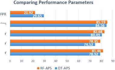
Fig.4. Performance parameters comparison

Several things can taint neuroimaging data, including variations in scanners, picture quality, and motion artifacts. The accuracy of the results and the data's variability can be influenced by these variables. In order to guarantee high-quality results, it is crucial to meticulously choose and assess the imaging procedures utilized in the study. A study's generalizability and reliability are greatly affected by the size of the size of the dataset. Large samples can be computationally costly and time-consuming, while small ones might result in overfitting and insufficient statistical power. Researchers should thus make sure the sample size is enough for the intended analysis after giving serious consideration to the sample size required to answer the research question. Performance parameters are analyzed and depicted in Fig 4.

Results precision and interpretability are both impacted by feature selection strategies. Not all feature selection approaches capture all aspects that are relevant to the situation at hand, and some may even be biased towards particular features. Hence, researchers need to assess several feature selection approaches for their effectiveness and pick the best one for the given situation. It is critical to be able to generalize the suggested procedures to other populations or datasets. When there are major variations in imaging processes or demographics, methods that work well on one dataset might not be able to transfer to another. Researchers should make sure the proposed approaches can be applied to new datasets or populations by carefully evaluating their generalizability. Table 1 shows a comparative analysis of existing machine learning algorithms and proposed ones.

Table 1. Performance analysis of various approaches

Model	Accuracy (%)	Precision (%)	Recall (Sensitivity) (%)	F1-Score (%)	AUC (Area Under Curve)	Interpretability	Training Time (s)
DT-APS (Proposed)	78.92	84.56	80.49	88.9	0.92	High	15
RF-APS (Proposed)	81.46	85.19	82.68	91.6	0.94	Moderate	20
Support Vector Machine	84.5	82.3	85.7	84	0.88	Low	30
k-Nearest Neighbors (k=5)	80.2	78.6	81.4	80	0.85	Low	12
Logistic Regression	82.1	80.4	82.8	81.6	0.87	High	8
Gradient Boosting Machine	87.3	85.2	88.6	86.8	0.91	Low	40
Deep Neural Network (DNN)	92.4	91	94	92.4	0.95	Very Low	150

Think of a dataset containing information on bridges, where each bridge type column has the values listed below. In order to comprehend label encoding, we will concentrate on a single category column, even though the data set will contain several more columns. We may directly normalize input variables in a dataset by using MinMaxScaler. The study will make use of the factory settings and scale all numbers to between 0 and 1. Set the default hyperparameters for the MinMaxScaler object before anything else. After the fit_transform() method is constructed, we can send it our dataset and use it to generate a transformed version of it.The reliability, particularity, accuracy, responsiveness, and false positive rate (FPR) of the suggested prediction model were assessed using the AQ-10 dataset in conjunction with real-world data. It is feasible to utilize the prediction algorithm created to advise undiagnosed people on potential autism symptoms. Either "User does not possess autism traits" or "User exhibits potential autism traits and demands comprehensive autism assessment" would be the model's recommendation for the user. Using the aforementioned factors, algorithms were evaluated and compared across three age groups: children, adolescents, and adults.

The algorithms' performance parameters were computed using AQ-10 datasets in accordance with the Leave-One-Out Technique. In this method, all data, apart from the instance being predicted, will be utilized as training data. The AQ-10 dataset is an established tool that uses answers to ten questions to determine the probability of autism spectrum disorder (ASD). Because of its ease of use and diagnostic value, it has been extensively utilized in both clinical and research contexts. 500 samples from the AQ-10 dataset, which was utilized in this investigation, range in age from 6 to 40 years and are evenly distributed by gender (50 percent female, 50 percent male). A varied representation of demographics was ensured by recruiting participants from both clinical and non-clinical settings throughout the United

Kingdom. 450 samples made up the final dataset after incomplete responses (those answering less than 80% of the questions) were eliminated before to analysis. To guarantee reliable model assessment, the data was divided into training (70%), validation (15%), and test (15%) sets after being standardized to a [0, 1] range. The AQ-10 dataset was chosen because it has a high association with clinical diagnoses of ASD, making it a trustworthy standard by which to assess the suggested machine learning models. Although the AQ-10 dataset is a useful tool, its applicability to larger populations may be constrained by its modest size and emphasis on self-reported characteristics. To overcome these limitations, future research might use bigger, multi-modal datasets.

In comparison to the other two models, the suggested prediction model outperformed them on all performance metrics. Similarly, for each participant group, the RF-APS outperformed the DT-APS. Once again, the suggested prediction model performed better with adults than with adolescents. When looking at RF-APS, we got the same outcome.

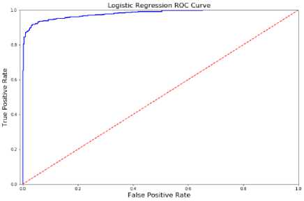
Fig.5. ROC curve analysis

While AQ-10 datasets of children, adolescents, and adults were utilized to train the prediction models, the 250 actual datasets were also used for model testing. Plotting performance metrics on a real-world dataset of children. Fig 5 shows a comparison of the ROC curve with the AQ-10 dataset values.

Fig.6. Validation loss

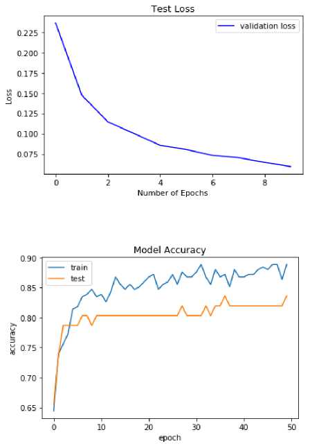
Fig.7. Training vs testing accuracy

Fig 6 shows the validation loss curve obtained during the training process. Although the actual dataset has a greater FPR than the AQ-10 dataset, it has worse accuracy, specificity, sensitivity, and precision. Since the prediction models were trained using the AQ-10 dataset and because the real data was acquired through surveys, it is possible that the respondents were not as serious as they claimed to be, leading to relatively poor performance in the real dataset. From the chosen datasets, the correlation between age distribution and autism spectrum disorder has been depicted in Figu.

In order to train and validate the system, we looked into the site-specific operating features by selecting samples from only one location. In order to assess the 10-fold CV, a minimum of 10 samples were needed; however, only 5 samples were chosen for the CMU site. Consequently, the CMU site was not included in this investigation.

Changes in intra-site performance as a function of sample size are also displayed. A larger validation sample may provide better results, whereas a smaller training sample may show worse results. This is the general norm. We did not discover a correlation between sample size and the accuracy of diagnoses, and we saw conflicting results. Since we only collected a small number of samples from each location, it would have been difficult to draw any conclusions on the correlation between sample size and precision. It is important to assess the age-specific performance of the suggested approach because of the heterogeneities that exist across various age cohorts. Figure 7 depicts training and testing accuracy analyses.

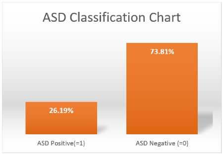
Fig.8. ASD classification analysis

Therefore, we separated the dataset into three age groups: kids, teens, and adults. Based on the patient's age when the MRI was taken, each subject is classified as either an adult, teenager, or kid. Cohorts for children and adolescents are defined by age ranges of less than ten and less than eighteen years old, and for adults, by age ranges of eighteen to sixty-four years old, respectively. All MRI samples taken from children fall into the children's cohort. The reason the suggested method works so well with children could be because the most striking variations in the local brain connections between the ASD and TC groups are shown in early life. Perhaps because the teenage group included both young and adult individuals, it performed worse across all three assessment parameters compared to the other two cohorts. ASD classification analysis is depicted in Figure 8.

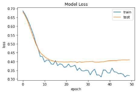
Fig.9. Model loss analysis

A further factor contributing to the increased heterogeneity in this group is the possibility of abnormal pubertal development in autistic children. As a result of different criteria for sample selection or the inaccessibility of every specimen for a given modality, the number of samples collected varies among researchers. Due to the inaccessibility of a whole dataset, we employed 857 out of 1500 samples. Since the two models are directly comparable, it follows that they were both trained and evaluated using the same data set consisting of the same people. Figure 9 depicts the model loss analysis obtained in the experimentation.

5.    Conclusions

In this paper, we propose a novel methodology leveraging the ML techniques DT-APS and RF-APS for automatic ASD identification. By focusing on features with high discriminatory power, our approach enhances identification accuracy while streamlining the training process of ML models. We introduce a picture descriptor utilizing a generalized Gaussian distribution (GGD) to reduce feature dimensionality, combined with the curvelet transform for multiscale representation. This allows for the characterization of brain regions in terms of both texture and shape, facilitating interpretability. Our method involves partitioning MRI scans into specific anatomical areas and representing them as adjacent slices in 2D images. Each image is then mapped to the curvelet space to extract characteristic features, with distinct curvelet sub-bands described by GGD parameters. Evaluation using the AQ-10 dataset demonstrates the efficacy of our proposed model. Across all metrics, including accuracy, specificity, sensitivity, precision, and false positive rate (FPR), our prediction model consistently outperforms alternative approaches. These findings underscore the potential of our methodology for revolutionizing ASD detection, offering a promising avenue for future research and clinical applications.