Unveiling Hidden Patterns: A Deep Learning Framework Utilizing PCA for Fraudulent Scheme Detection in Supply Chain Analytics

Published Online on April 8, 2025 by MECS Press

Supply Chain Management (SCM) is a strategic approach to overseeing the entire lifecycle of goods and services, from their creation or acquisition to their delivery to the end consumer. SCM involves the coordination of various activities, including procurement, production, transportation, warehousing, and distribution, to optimize the overall efficiency and effectiveness of the supply chain. Every company, no matter its size or industry, relies on these networks to function well. Yet, fraud may also occur in supply networks, and this can have a major monetary effect on companies. In a 2020 report of Word Economic Forum (WEF), companies lose trillions of dollars annually due to supply chain fraud. PwC Global Economic Crime Survey 2022 reports that 57% of fraud is committed by insiders or a combination of insiders and outsiders, leading to losses of $50 billion annually for businesses. This includes losses from procurement fraud, employee theft, and other forms of supply chain fraud. However, operational interruptions, reputational harm, legal expenses, and so forth are all forms of SCM losses that can result from fraud. Within the vast landscape of SCM, fraudulent schemes represent a persistent and challenging threat. Fraud in the supply chain can manifest in various ways, including but not limited to misrepresentation of products, theft, counterfeiting, and deceptive practices in transactions. These schemes often exploit vulnerabilities in the complex web of interconnected processes, making detection and prevention critical for maintaining the integrity of the supply chain.

The importance of early detection of fraudulent schemes in SCM cannot be overstated. Timely identification allows for swift intervention and mitigation of potential damages. Financial losses, reputational damage, compromised product quality, and disruptions in the supply chain can be averted or minimized when fraudulent activities are detected early. Detecting fraudulent schemes early requires a proactive and technology-driven approach. Advanced tools and techniques, such as data analytics, machine learning, and deep neural networks, play a pivotal role in uncovering anomalous patterns and behaviors indicative of fraudulent activities. By leveraging these technologies, organizations can establish robust monitoring systems that enhance the resilience of the supply chain against fraudulent threats, ultimately safeguarding both economic interests and consumer trust. Several different approaches are used to detect fraud in the supply chain. These approaches can be broadly divided into two categories, Rule-based approaches and AI based techniques.

Rule-based methodologies are frequently rigid and might provide challenges in staying abreast of the most recent fraudulent techniques. Furthermore, manual fraud detection approaches have a poor level of accuracy, making it exceedingly challenging to manage substantial amounts of data. Machine learning, a branch of artificial intelligence, offers a potential approach to improve the identification and prevention of fraud in complex supply chain networks. Machine learning has the capacity to detect fraudulent trends and adapt to new and complex types of fraudulent behaviors by utilizing advanced algorithms, predictive modeling, and data analytics. Machine learning or deep learning methods can yield superior results, but they want substantial quantities of high-caliber data for training and possess the capability to uncover concealed patterns. Historically, the fraud detection process relied mostly on audit approaches that were deemed inefficient [1]. Nevertheless, in recent times, corporations have relied on Artificial Intelligence (AI) technology, particularly machine learning (ML) systems [2].

The motivation behind this research stems from the critical importance of securing global supply chains against fraudulent practices. As traditional fraud detection mechanisms struggle to keep pace with the ever-evolving tactics employed by fraudsters, there arises a need for a proactive and intelligent approach that can learn from historical data, recognize anomalies, and continuously improve its effectiveness. In this paper, we propose a novel deep learning framework for fraud detection in supply chain analytics incorporating principal component analysis. Our proposed framework uses a deep neural network to learn complex patterns in data from a variety of sources, including order details, customer information, and shipment information. The framework is able to detect fraudulent transactions with high accuracy and detection rate, even in cases where the fraud is complex or novel. The overall contributions of this work confined intro three segments are stated below:

• •    In order to detect fraudulent activity in supply chain networks, a unique deep learning architecture has been proposed.

• •    Principal component analysis has been employed to reduce high-dimensional data into an optimal collection of features along with deployment of Bayesian optimization method for hyper-parameter fine tuning. Throughout our effort, the working model avoids the curse of dimensionality problem.

• •    To address the class imbalance problem, SMOTE has been used to oversample the minority class, enhancing the model’s ability to detect fraudulent activities effectively.

• •    For the purpose of assessing the operational performance of our proposed framework on a benchmark dataset, a set of evaluation metrics has been deployed.

• •    To validate the robustness and superiority of the proposed model, performance metrics have been compared across a set of individual ML and deep learning classifiers along with the state-of-the-art models in the supply chain analytics.

2.    Literature Review

The remaining sections of the paper have been organized in the following manner. Section 2 provides a discussion of the works that are related to the topic. Section 3 presents the comprehensive structure of our proposed model, together with a description of the associated dataset. Section 4 provides a comprehensive overview of all the experimental assessments employed in this study. Section 5 pertains to the experimental settings, whereas Section 6 encompasses the essential experimental results and debates of the whole paper. At last, we have reached the conclusion of our effort in Section 7.

The fraud detection technology in financial services can be divided into two major categories: Rule based methods and machine or deep learning techniques.

Rule-based methodologies employ a predefined set of rules to detect transactions that are prone to being fraudulent. For instance, a rule could identify a transaction as fraudulent if the order value is abnormally elevated or if the supplier is not listed among the company's authorized vendors. Furthermore, it necessitates costly and proficient domain expert teams and data scientists. Frequently, it necessitates rigorous inquiries into the additional transactions associated with deceitful behavior in order to discern patterns of fraudulent activity. Finance businesses are not achieving sufficient return on investment (ROI) despite the allocation of resources and funds towards these conventional approaches.

The authors of [3] introduce the financial fraud modelling language, FFML, which is a rule-based policy modeling language and comprehensive architecture. It allows for the conceptual expression and implementation of proactive fraud protection in multi-channel financial service platforms. The work demonstrates the use of a domain-specific language to streamline the financial platform by converting it into a data stream-oriented information model. The objective of this technique is to reduce the intricacy of policy modeling and limit the duration required for policy implementation. It does this via the employment of a new policy mapping language that can be utilized by both expert and non-expert users. The Improved Firefly Miner, Threshold Accepting Miner, and Hybridized Firefly-Threshold Accepting (FFTA) based Miner are new rule-based classifiers that use Firefly (FF) and Threshold Accepting (TA) algorithms. These classifiers are designed to determine if a company's financial statements are fake or not. The authors examine how t-statistic-based feature selection affects outcomes. Both FFTA and TA miners were statistically comparable. According to [4], the two algorithms fared better than the decision tree in terms of sensitivity and rule length. In the study [5] introduced a twotiered framework for detecting credit card fraud. This framework incorporates both a rule-based component and a game-theoretic component. The utility of classical game theory lies in its ability to determine optimal strategies regardless of the actions taken by the opponent, hence obviating the necessity for prediction. The study conducted by [6] investigated the impact of fraud intention analysis on quality inspection. Suppliers and purchasers may engage in several transactions, including with potential fraudsters, in order to gather information about each other during the process of quality inspection. The supply contracts may also affect the profit-seeking behavior of providers. The researchers conducted experiments in a laboratory to evaluate the effectiveness of fraud intention analysis systems on decision making during inspections. They specifically examined the impact of learning and contract effects. The experiment was conducted on a dairy supply chain, which was both fascinating and essential. The experiment shown that analyzing fraud intention might enhance the efficiency of buyers' decision-making, taking into account factors such as decision time, inspection cost, and accuracy in rejecting suppliers' fraudulent shipments, provided that the contract lacks severe repercussions for fraud. The majority of traditional fraud detection approaches mostly concentrated on discrete data points. Nevertheless, these approaches are no longer enough for the demands of the present day. As fraudsters and hackers employ increasingly sophisticated and innovative methods to conceal their fraudulent actions, even from the most discerning observers. To overcome the limitations of standard approaches, an analytical approach is necessary as these methodologies can only identify known attack types [7].

Insufficient capacity to manage large volumes of big data and address financial fraud adequately can result in significant losses within supply chains [8]. To solve the problem of handling high dimensional data, many companies inclined to ML or deep learning techniques along with different platforms like Apache spark, Hadoop and so on. Artificial intelligence (AI) is being widely employed in supply chain management with big data to effectively identify and prevent fraudulent behavior [9-11].

The real-time application benefits from the efficient and effective outcomes provided by machine learning techniques. Several techniques have been used to achieve the desired outcomes. XGBoost, LR, RF, and DT are the most often used techniques [12]. In contrast to earlier writers that employed conventional techniques, in [13] developed an ensemble model that utilizes deep recurrent neural networks, and a distinctive voting mechanism based on artificial neural networks to detect fraudulent transactions. The model is specifically designed for sequential data modeling. Two real-world datasets were used by the authors to illustrate the suggested work. The transaction data that represented the behavior of the customers was collected and analyzed by [14]. They combined deep learning techniques with the machine learning approach, rather than relying only on it. In recent times, businesses have become reliant on machine learning systems and artificial intelligence (AI) technologies.

A study examined five distinct supervised learning approaches, including LR, MLP, Boosted Tree, RF and SVM. Upon comparing the results, the boosted tree model demonstrated the highest efficacy in detecting fraud, achieving a 49.83% fraud detection rate for the specified dataset [15]. SVM with a specialized financial kernel was used for management fraud detection in [16]. Leveraging basic financial data, the SVM model correctly classified 80% of fraudulent cases and 90.6% of legitimate cases on a holdout set. This highlights the efficacy of SVMs in discerning fraudulent patterns and underscores the potential of this approach in enhancing current fraud detection strategies. In another study of fraud detection in credit card transactions, the XgBoost algorithms exhibits a high AUC of 0.99, but moving towards its peak may increase false positives, risking misclassification [12]. The authors of [17] introduce a machine learning framework for predicting fraudulent activities within Supply Chain links, employing RF, KNN, and LR algorithms. The optimal model is enhanced through grid search cross-validation, demonstrating increased efficiency with a 97.7% accuracy score. In another study of credit card fraud detection LR, RF, Naive Bayes (NB), and Multilayer

Perceptron (MLP) algorithms, revealing their high accuracy. The proposed model in [18] extends applicability to detecting various irregularities. In [19], authors presented SVM as better model comparing LR and Naïve Bayes with 98.61% overall classification accuracy by using DataCo supply chain dataset. The authors of [20] presented two data-driven methodologies that enhance decision-making in supply chain management. The proposed anomaly detection technique for multivariate time series data shows superior performance when utilizing the LSTM Autoencoder network, particularly in the context of supply chain management. The DataCo Supply Chain Dataset for Bigdata Analysis was used in [21] for developing fraud detection hybrid model incorporating XgBoost and Random Forest algorithms. The authors of [8] proposed a distributed big data mining for supply network financial fraud detection. The method uses a distributed deep learning model, CNN. It uses Apache Spark and Hadoop's big data technology. This method speeds up parallel processing of large datasets to substantially reduce processing times. The proposed method intelligently classifies huge data samples using training and testing on the continuously updated Supply Chain Finance (SCF) dataset to detect fraudulent financing operations. This study develops and runs CNN, SVM, and Decision Tree algorithms using Apache Spark. During repeated training, the CNN model detects more financial fraud cases and less normal samples as false positives. CNN model's highest accuracy is about 93% and average precision is above 91% and consistently outperforms the other two models. These findings enhance distributed deep learning research for supply chain financial fraud detection.

In addition to the related works previously discussed, various studies have been conducted in financial fraud detection; however, there is limited research focusing on supply chain management with the application of different deep learning techniques. The potential benefits of developing a deep learning model that incorporates multiple layers with appropriate activation functions and regularization are not yet well recognized in this field. To address the challenges of class imbalance and high-dimensional feature complexity, our approach includes oversampling to mitigate bias in the majority class and feature engineering to manage computational demands. These strategies are aimed at developing an effective deep neural network model for fraud detection in our research.

3.    Proposed Approach

In this paper, we introduce a novel hybrid method for detecting fraudulent transactions in the supply chain using a deep neural network (DNN) with a focus on principal component analysis (PCA). To facilitate a comprehensive understanding of our proposed approach's workflow and architecture, this section is organized into four sequential subsections. Sub-section 3.1 provides an overview of our proposed model and its general architecture. Sub-section 3.2 delineates the characteristics of the dataset utilized in this study. The pre-processing unit of our model, addressing feature transformation and dimensionality reduction, is thoroughly explained in sub-section 3.3. Finally, sub-section 3.4 delves into the detailed analysis of the model designed for identifying fraudulent schemes, succinctly outlining each fundamental element of the overall model.

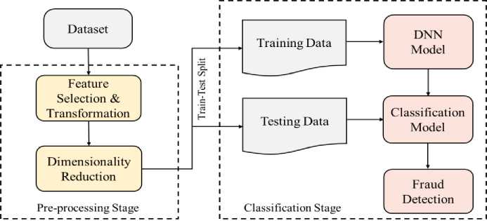
Fig. 1. Overview of proposed architecture

• 3.1.    Proposed Architecture

• 3.2.    Dataset Description

• 3.3.    Data Cleaning and Preprocessing

Illustrated in Fig. 1, our proposed model comprises two core components: a pre-processing unit and a DNN model for the classification phase. The initial segment of the pre-processing unit handles feature transformation, beginning with the removal of irrelevant features. Each ordinal feature is then converted into a label-encoded format, representing each input byte as an n-dimensional vector. Subsequently, a data standardization operation is applied after numerical representation conversion. The second segment involves a dimensionality reduction unit aimed at addressing the curse of dimensionality. PCA serves as the foundation for this feature reduction operation. Utilizing PCA, the chosen features from the datasets are transformed into a specific number of principal components, from which only a selected few are retained for the detection model. This process is consistent for both the training and testing datasets. Following the completion of the pre-processing unit, the reduced and transformed features are directed into the DNN model, which plays a pivotal role in fraud transaction detection.

In order to assess the efficacy and dependability of any fraud detection technology, a proficient dataset is required. An effective dataset comprises a substantial quantity of precise data that accurately represents actual networks in the real world. We have utilized the well-recognized public supply chain dataset called DataCo SMART SUPPLY CHAIN FOR BIG DATA ANALYSIS for our research in this article. The dataset has collected from Mendeley that was created to help people understand how big data can be used to improve supply chain efficiency [22]. There are three main types of data present in this dataset: structured data, unstructured data, and descriptive data. The dataset contains data on orders, shipments, and customers from a large e-commerce company. This data can be used to analyze trends in customer behavior, identify areas for improvement in the supply chain, and optimize the company's logistics operations. It can be used to improve the efficiency, effectiveness, and profitability of supply chains. Table 1 illustrates the description of the dataset. However, one of the key drawbacks of this dataset is that it is imbalanced, containing a large number of legitimate labels compared to fraud labels. This imbalance can cause bias towards the majority class, often leading to poor performance in predicting the minority class. The model tends to prioritize accuracy on the majority class, which can dominate the loss function.

Table 1. List of variables with data types

SL No.	FIELDS	TYPES OF VARIABLES	SL No.	FIELDS	TYPES OF VARIABLES
1	Type	Categorical	28	Order Customer Id	Id
2	Days for shipping (real)	Numerical	29	Order date (Date Orders)	Date-Time
3	Days for shipment (scheduled)	Numerical	30	Order Id	Id
4	Benefit per order	Numerical	31	Order Item Cardprod Id	Id
5	Sales per customer	Numerical	32	Order Item Discount	Numerical
6	Delivery Status	Categorical	33	Order Item Discount Rate	Numerical
7	Late_delivery_risk	Numerical	34	Order Item Id	Id
8	Category Id	Id	35	Order Item Product Price	Numerical
9	Category Name	Categorical	36	Order Item Profit Ratio	Numerical
10	Customer City	Categorical	37	Order Item Quantity	Numerical
11	Customer Country	Categorical	38	Sales	Numerical
12	Customer Email	Text	39	Order Item Total	Numerical
13	Customer Fname	Text	40	Order Profit Per Order	Numerical
14	Customer Id	Id	41	Order Region	Categorical
15	Customer Lname	Text	42	Order State	Categorical
16	Customer Password	Id	43	Order Status	Categorical
17	Customer Segment	Categorical	44	Order Zip code	Numerical
18	Customer State	Categorical	45	Product Card Id	Id
19	Customer Street	Categorical	46	Product Category Id	Id
20	Customer Zip code	Id	47	Product Description	Text
21	Department Id	Id	48	Product Image	Text
22	Department Name	Text	49	Product Name	Text
23	Latitude	Numerical	50	Product Price	Numerical
24	Longitude	Numerical	51	Product Status	Categorical
25	Market	Categorical	52	Shipping date (Date Orders)	Date-Time
26	Order City	Categorical	53	Shipping Mode	Categorical
27	Order Country	Categorical

Table 1 reveals that the dataset comprises 53 variables or features of varying data types and Fig. 2 demonstrates the count of different types of variables.

In our dataset, the pre-processing stage encompasses two consecutive steps: feature selection and transformation, followed by dimensionality reduction.

Several redundant variables have been eliminated from the dataset. Variables related to customer demographics, such as 'Customer Email,' 'Product Status,' 'Customer Password,' 'Customer Street,' 'Customer Fname,' 'Customer Lname,' 'Customer Zipcode,' 'Product Description,' 'Product Image,' and 'Order Zipcode,' have been removed, as they wouldn't contribute to creating classification models. Additionally, numeric variables serving as unique IDs for departments or products, including 'Category Id,' 'Customer Id,' 'Department Id,' 'Order Customer Id,' 'Order Id,' 'Order Item Cardprod Id,' 'Order Customer Id,' 'Order Item Id,' 'Product Card Id,' and 'Product Category Id,' have been excluded from the dataset. Furthermore, 'order date (Date Orders)' and 'shipping date (Date Orders)' variables have been dropped as the year, month, and day have already been extracted for use in the model.

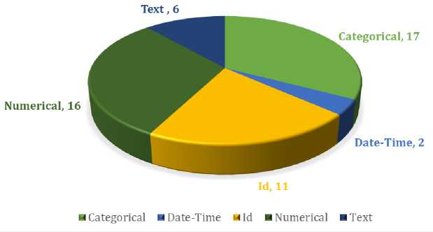
Fig.2. Breakdown of variable types

In this stage of pre-processing, both numericalization and standardization of the data have been implemented. To address the limitation of machine learning algorithms in handling categorical features, numericalization of the data was prioritized in the initial steps. As the dataset contains 17 categorical features, label encoding was employed to convert non-numeric values into a numeric format. Although one hot encoding is another commonly used method for this purpose, it has the drawback of generating a substantial number of new dimensions by assigning binary vectors to nominal data.

After selecting the relevant features, the dataset has been split into training and testing sets with a ratio of 80% to 20% where random seed is 42. Before feeding the data into the model, we labeled the "Suspected_Fraud" transactions as 1 and the rest of the "Order Status" transactions as 0, indicating legitimate transactions. The count of two kinds of transactions in the supply chain has been shown in Table 2 along with breakdown of label data of train and test set.

Table 2. Number of records of each class

Order Status	Total	Train Data	Test Data
Legitimate	176457	141203	35254
Fraud	4062	3212	850

Table 2 highlights a severe class imbalance between the "Legitimate" and "Fraud" classes. Both train data and test data consist of approximately 98% legitimate transactions and 2% fraudulent transactions. When a machine learning model is trained on such highly imbalanced data, where legitimate transactions vastly outnumber fraudulent ones, it often becomes biased toward predicting the majority class. This can result in high accuracy but poor detection (sensitivity) of fraudulent transactions, which is critical in fraud detection. The lack of sufficient examples from the minority class can lead to difficulties in identifying fraud and hinder the model's ability to generalize to unseen data, ultimately reducing its effectiveness in real-world scenarios.

To address this class imbalance, oversampling techniques such as SMOTE (Synthetic Minority Over-sampling Technique) has been applied to the training data. SMOTE generates synthetic examples of the minority class, in this case, fraudulent transactions, thus making the training set more balanced. This approach enables the model to better learn the characteristics of fraudulent transactions by providing more examples from the minority class. Additionally, a balanced training set improves performance metrics such as recall, precision, F1-score, and AUC-ROC for the minority class, which are critical for effective fraud detection. Furthermore, oversampling helps mitigate the bias toward predicting only the majority class, thereby enhancing the model’s ability to detect fraud accurately. Fig. 3 illustrates the distribution of product prices by order status. The first image highlights the class imbalance problem, while the second image shows the balanced classes after oversampling the ‘Fraud’ class.

The heatmap of Fig. 4 represents the correlation or strength of the relationship between each feature. Here it can be seen that the number of high correlated variables are comparatively low, which is good for the classification model. Low correlation suggests that each variable contributes unique and independent information to the model, allowing it to capture a broader range of patterns and relationships in the data. This independence can lead to improved model performance, as the variables provide diverse perspectives and avoid introducing multicollinearity issues. Additionally, low correlation enhances the interpretability of the model, as the influence of each variable can be more easily discerned, facilitating a better understanding of the underlying features driving the classification outcomes.

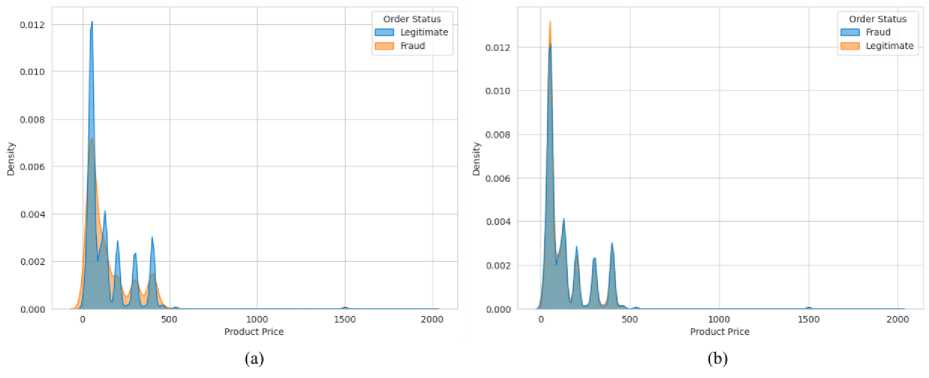
Fig.3. Distribution of Product Price by Order Status (a) before oversampling (b) after oversampling

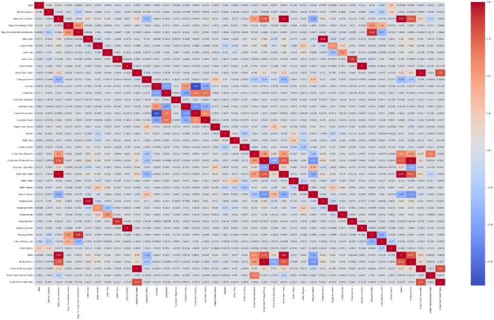
Fig.4. Heatmap of correlated variables

The objective of feature scaling is to bring all features in the dataset to a nearly equal scale, facilitating analysis by most machine learning algorithms. In this study, standardization was chosen for feature scaling, proving to be more effective than the traditional min–max normalization approach. Following label encoding, standardization was implemented to rescale all features, ensuring a mean of 0 and a standard deviation of 1, resulting in a distribution that is centered around zero and has a consistent scale. This makes it easier for machine learning algorithms to converge and perform well, especially in cases where features have different units or magnitudes. The formula is expressed as follows in Eq 1:

S

x - mean ( x )

std ( x )

where std means standard deviation, s is the standardized value of the feature and x represents original value of the feature.

A lot of research has shown that the ability of any classifier to predict things gets better as the number of variables of the training samples rises. But work starts to fall apart after a while. Because of this, the event is called the "curse of dimensionality" [23-25]. For the purpose of getting rid of this problem in our model, PCA has been used. It helps reduce the size of the information to a level that you want. Once the main parts of the real features have been found, the variation level of each feature has been used to choose the smallest number of features. In this way, the model stays free of any very high levels of complexity. One quick look at the model's pre-processing stage can be seen in Fig. 5.

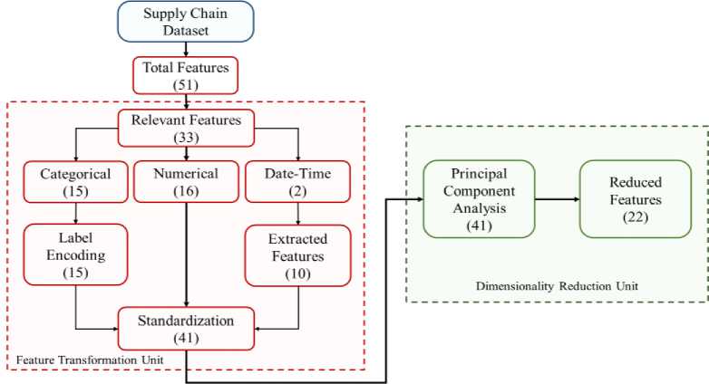
Fig.5. The procedural flow during the pre-processing stage

PCA is a method that doesn't rely on class labels to identify the most important features in a dataset. This means that the components found by PCA will be the same regardless of how the data is labeled. The importance of a component is determined by how much of the variation in the data it explains. We chose PCA for dimensionality reduction primarily due to its ability to effectively capture the variance in the data while reducing the dimensionality. PCA is particularly well-suited for identifying the directions (principal components) along which the data varies the most, which helps in simplifying the dataset while preserving as much information as possible. Compared to other dimensionality reduction techniques, PCA was favored for its simplicity and ease of implementation, especially given the linear nature of our data. In this work, the number of components was determined by analyzing the cumulative explained variance ratio. We selected the number of components that captured 90% of the total variance, ensuring that

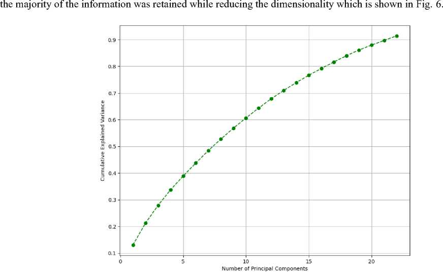
Fig.6. Cumulative explained variance for PCA components

• 3.4.    Deep Neural Network

After using PCA to reduce the number of features, a deep neural network was created to classify the data. The reduced set of features was used as the input to the neural network. We selected deep learning for this study because of its ability to automatically learn complex patterns and representations from data, especially in scenarios where the data has high dimensionality. Traditional machine learning models, while effective for certain tasks, often require extensive feature engineering, which deep learning models can bypass by learning hierarchical features directly from the raw data. However, overfitting is a significant concern with deep learning models, especially when dealing with smaller or imbalanced datasets. To address this, we employed regularization techniques, such as dropout, to manage the overfitting problem to ensure effective performance from the model. The deep neural network consists of four fully connected layers, and the final layer uses a sigmoid function to activate the output. The details of the parameters of the neural network are provided in Table 3. To manage the computational cost, we utilized optimized hardware and implemented techniques such as early stopping to minimize unnecessary computational overhead. To mitigate concerns regarding computational overhead, we implemented optimization techniques such as hyperparameter tuning to improve efficiency. The Bayesian optimization approach has been employed to optimize the essential hyperparameters in the model, aiming to improve efficiency and streamline the process. Bayesian Optimization uses probabilistic models to explore the hyperparameter space more intelligently. It builds a surrogate model of the objective function and selects hyperparameters by optimizing an acquisition function. It is more sample-efficient than other techniques like Grid and Random Search, requiring fewer evaluations to find optimal or near-optimal hyperparameters. The remaining details of the model are outlined in sub-section 3.4.1.

Table 3. Bayesian optimized parameters for the deep learning classifier

Hyper-Parameters	Functions/ Values
Dense Layer (1)	Activation = ReLu, Neurons = 512
Dense Layer (2)	Activation = ReLu, Neurons = 128
Dense Layer (3)	Activation = ReLu, Neurons = 64
Dense Layer (4)	Activation = Sigmoid, Neurons = 1
Dropout	0.2
Learning Rate	0.001
Cost Function	Binary Cross Entropy
Batch Size	64
Optimizer	Adam
Iterations	50

Dense Layer

A dense layer, commonly referred to as a fully connected layer, is an essential component in deep neural networks. Each neuron in a layer is linked to every neuron in the subsequent layer, which is a defining characteristic. The term "dense" refers to the dense connections between neurons. The architecture of a dense layer involves weights and biases, which are parameters that the neural network learns during the training process [26-27].

Here's a more detailed breakdown of the dense layer architecture:

• •    Neurons/Nodes: Each node in a dense layer represents an artificial neuron. The number of nodes in a dense layer is the layer's width or size.

• •    Weights: Each connection between neurons in adjacent layers has a weight associated with it. Weights refer to parameters that the neural network acquires through the training process, and they play a crucial role in determining the intensity of connections between neurons.

• •    Biases: Every neuron in a dense layer is associated with a bias. Biases allow the model to account for situations where all input features are zero.

• •    Activation Function: Each neuron typically has an activation function that introduces non-linearity to the network. The sigmoid, the rectified linear unit (ReLU), and the hyperbolic tangent (tanh) are all common activation functions.

• •    Forward Pass: During the forward pass, input data is multiplied by weights, and the biases are added to the result. The sum is then passed through the activation function to introduce non-linearity.

• •    Training: During training, the weights and biases are adjusted using optimization algorithms such as gradient descent. The model learns to minimize the difference between its predictions and the actual target values.

• •    Backpropagation: Backpropagation is the process by which the neural network adjusts its weights and biases based on the error calculated during training. This process entails calculating the gradients of the loss function in relation to the weights and biases, and subsequently adjusting them based on these gradients.

4.    Experimental Setup 5.    Evaluation Metrics

The architecture of deep learning models often involves stacking multiple dense layers along with other types of layers like convolutional layers and recurrent layers. This hierarchical structure allows deep neural networks to learn complex hierarchical representations of data, capturing intricate patterns and relationships. The fundamental dataflow diagram of dense layer architecture is represented in Fig. 7.

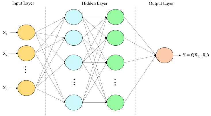
Fig.7. Dense layer architecture

Given the exhibited class imbalance in the dataset and the presence of highly collinear features, employing a Deep Neural Network (DNN) is considered a suitable choice to address the problem. Deep neural networks (DNNs) can address data imbalance and multicollinearity issues through their inherent capacity to learn hierarchical representations of data. In the case of data imbalance, DNNs can adaptively assign different weights to under-represented classes during training, mitigating the bias towards the majority class. Additionally, techniques like oversampling and under sampling can be integrated into the training process. Regarding multicollinearity, the deep architecture of neural networks enables them to automatically extract relevant features and hierarchies, reducing the impact of redundant or highly correlated input features. This intrinsic ability to learn complex relationships allows DNNs to handle imbalanced datasets and multicollinear features, making them robust and effective in various real-world applications.

The research that was done for this work was done using the programming language Python, especially version 3.6.9. Python tools that are often used, like Pandas and Numpy, were used to analyze the data. Keras, a deep-learning API that works on the Tensorflow platform, was used to put deep learning models into action. Using a TPU, all tasks related to the project were done on Google Colaboratory.

The assessment of a model's effectiveness in any detection system depends on its evaluation metrics, specifically the confusion matrix. This matrix serves as a comprehensive representation of a classification algorithm's performance, offering essential relative information. For his study, four widely recognized performance metrics—Accuracy, Precision, F1-Score, and Recall—have been extracted from the confusion matrix of the detection model.

Predicted Class
i rue ^1аъъ	Legitimate	Fraud
Legitimate	TN	FP
Fraud	FN	TP

Fig.8. Confusion matrix

Fig. 8 illustrates the confusion matrix, delineating four potential outcomes. The analysis of overall results is based on these outcomes, and it involves the utilization of the four most commonly employed evaluation metrics:

• •    TN (True Negative): Instances of legitimate correctly classified by the classifier.

• •    FP (False Positive): Instances of legitimate misclassified by the classifier.

• •    FN (False Negative): Instances of fraud misclassified by the classifier.

• •    TP (True Positive): Instances of fraud correctly classified by the classifier.

• I.    Accuracy: Determines the proportion of correctly classified test instances relative to the total number of test instances.

TP + TN

Accuracy =----------------

TP + TN + FP + FN

• II.    Precision: Measures how many instances that were predicted as positive were actually positive.

  Precision =

  
  

  TP

  TP + FP

  
  
  
  

• III.    Recall (Detection Rate, True Positive Rate): The proportion of positive instances in the test set that were accurately identified in relation to the overall count of positive instances.

  Recall =

  
  

  TP

  TP + FN

  
  
  
  

• IV.    F1 Score: The harmonic average of precision and recall is interpreted, creating a balance between the two measurements.

6.    Result Analysis

• 6.1.    Phase 1: Results of Classification Using Both the Actual and Reduced Features

2* Recall * Precision

F 1 =------------------

Recall + Precision

These metrics are frequently employed to evaluate the efficacy of a classification model, especially in tasks like fraud transaction detection where correctly identifying positive instances (fraud) is crucial, and balancing precision and recall is important.

The performance of the supply chain fraud transaction detection model is gauged by its evaluation metric scores. In an effort to make the findings of this study more understandable, they have been divided into two distinct parts. Performance criteria for binary classification are outlined in the first phase (Phase 1) of the segment. After that, Phase 2 provides a comparative study of the total findings, taking into account individual machine learning and deep learning classifiers in addition to models that are considered to be state-of-the-art in the relevant sector.

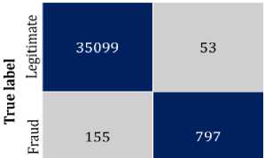
In order to distinguish between fraudulent and legitimate transactions, binary classification has been implemented. The confusion matrix for both actual and reduced features is illustrated in Fig. 9. The scores of the four metrics, which are derived from the confusion matrix, are presented in Table 4.

Legitimate

Fraud

Fraud

Predicted label

Predicted label

(a)

(b)

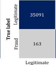
Fig.9. Confusion matrix of the classification model with (a) actual features (b) reduced features

The confusion matrix for the fraud detection model is depicted in Fig. 9. In Fig. 9(a) and (b), the confusion matrix for the model is shown with actual and reduced features, respectively. As indicated in Table 2, the order status variable exhibits class imbalance. To address this, we have applied the SMOTE technique to oversample the minority class. We then evaluated our proposed model using four key metrics, focusing primarily on the fraud detection rate due to the model's objective of early fraud detection in the supply chain. These metrics, derived from the confusion matrix, are summarized in Table 4. The model has been assessed both before and after applying PCA. The performance comparison between the models with and without PCA reveals that while both approaches achieve the same accuracy of 99.42%, there are subtle differences in other metrics. Precision, which measures the proportion of true positive predictions among all positive predictions, is slightly higher in the model without PCA at 83.72%, compared to 83.16% with PCA. This indicates a marginally better performance in correctly identifying positive instances without PCA. However, when it comes to recall, or the detection rate, the model with PCA performs better, achieving a 94.71% recall compared to 93.76% without PCA. This suggests that the model with PCA is more effective in identifying true positive cases overall. The F1-Score, which balances precision and recall, is almost identical for both models, with 88.56% for PCA and 88.46% without PCA, indicating that both approaches provide a similar balance between precision and recall.

Table 4. Comparison of performance between actual and reduced features

Measure	With PCA (%)	Without PCA (%)
Accuracy	99.42	99.42
Precision	83.16	83.72
Recall/ Detection Rate	94.71	93.76
F1- Score	88.56	88.46
Training Time (Seconds)	2715	3350
Testing Time (Seconds)	85	128

Another key observation of our work is that we acknowledge that simpler models with reduced deep learning layers can be advantageous in terms of interpretability and computational efficiency. In our study, we conducted preliminary experiments comparing the performance of several simpler models with our deep learning approach. Although some simpler models achieved comparable results, our proposed deep neural network consistently outperformed them in terms of accuracy and robustness, particularly on more complex aspects of the dataset.

In terms of computational efficiency, PCA demonstrates a clear advantage. The training time is significantly reduced from 3350 seconds without PCA to 2715 seconds with PCA, and the testing time is also faster with PCA, taking only 85 seconds compared to 128 seconds without PCA. Moreover, the training and testing times with employing PCA has been significantly lower due to dimensionality reduction, achieving a reduction rate of 46.34%. This highlights PCA's role in enhancing the model's efficiency while maintaining comparable performance across key metrics. Another key observation of our work is that we acknowledge that simpler models with reduced deep learning layers can be advantageous in terms of interpretability and computational efficiency. In our study, we conducted preliminary experiments comparing the performance of several simpler models with our deep learning approach. Although some simpler models achieved comparable results, our proposed deep neural network consistently outperformed them in terms of accuracy and robustness, particularly on more complex aspects of the dataset.

ROC curve

---WITH PCA(AUC = 0.9983)

--- WITHOUT PCA (AUG = 0.9980)

0.0               0.2               0.4                0.6                0.8               1.0

False Positive Rate

Fig.10. ROC curve for the classification model

The Receiver Operating Characteristic (ROC) curve is another useful tool for evaluating the performance of the classifier, especially in situations like imbalanced class distribution. The ROC curve is a graphical representation of the performance of a binary classification model at various threshold settings. It illustrates the trade-off between the true positive rate (sensitivity or recall) and the false positive rate (1 - specificity) as the discrimination threshold is varied. In Fig. 10, the observation comes from the ROC curve which indicates that when our model incorporates PCA, it covers a slightly larger area compared to the model that doesn't use PCA. The ROC-AUC score of the model with reduced features surpasses that of any other conventional machine learning and deep learning models due to its high fraud detection rate. Nevertheless, in both categories, the balance between the true positive rate (TPR) and false positive rate (FPR) at various threshold values demonstrates exceptional performance.

• 6.2.    Phase 2: Comparisons of other Approaches with Statistical Significance Test and Earlier Works

In order to demonstrate the efficacy of the proposed model in a wider scope, the complete procedure has been replicated for several conventional machine learning and deep learning classifiers. For this instance, there are no modifications made to any of the preparatory phases in the entire procedure. It has been shown in Table 5 that a comparison has been made between the proposed fraud detection model and other conventional models. The table compares the performance of various machine learning models in terms of overall accuracy and their ability to detect fraudulent activities. Among the models, the Random Forest model demonstrated the highest overall accuracy at 99.47% with a solid fraud detection rate of 81%. This is closely followed by the Decision Tree model, which achieved an accuracy of 99.21% and a slightly better fraud detection rate of 82%. Both models are strong performers in identifying fraudulent schemes, making them reliable options for such tasks. In contrast, the Logistic Regression, Support Vector Machine, K-Nearest Neighbors, and Gaussian Naive Bayes models had lower fraud detection rates, despite having relatively high overall accuracy. For example, the SVM model achieved 98.11% accuracy but only detected 30% of fraudulent activities. Similarly, the KNN model, with an accuracy of 98.02%, detected just 20% of fraud cases, while the GNB model, despite having 97.64% accuracy, completely failed to detect any fraudulent cases (0% detection rate). These results indicate that while these models perform well overall, they struggle with the specific task of fraud detection. Neural network-based models like the Multi-Layer Perceptron, Long Short-Term Memory, and Gated Recurrent Unit show varying results. The MLP model achieved an accuracy of 98.81% with a respectable fraud detection rate of 70%, making it a viable option for fraud detection. However, the LSTM and GRU models significantly underperformed, with both showing low overall accuracy (12.80% for LSTM and 12.05% for GRU) and equally poor fraud detection rates (11% and 10%, respectively). The proposed approach outperformed all other models in fraud detection, achieving a 95% detection rate while maintaining a high overall accuracy of 99.42%. This indicates that the proposed model is highly effective in identifying fraudulent activities, making it the most reliable choice among the models evaluated. Its superior performance in fraud detection, combined with its competitive accuracy, highlights its potential for real-world applications where identifying fraud is critical.

Table 5. Comparison of the proposed classifier model to others

Model	Overall Accuracy (%)	Fraud Detection Rate (%)
RF	99.47	81
LR	97.75	19
DT	99.21	82
SVM	98.11	30
KNN	98.02	20
GNB	97.64	00
MLP	98.81	70
LSTM	12.80	11
GRU	12.05	10
Proposed Approach	99.42	95

Friedman Test : The Friedman test is a non-parametric statistical test used for comparing multiple related samples. It is designed to determine whether there are statistically significant differences in the distribution of scores among different groups or treatments. The Friedman test was selected in our work because it is a non-parametric test specifically designed to compare multiple models across different conditions without assuming a normal distribution of the data. In fraud detection, the data is often skewed, with a large imbalance between legitimate and fraudulent cases. The Friedman test is robust to these conditions, making it well-suited for comparing the performance of different fraud detection models under these non-normal, imbalanced circumstances. While the results of the Friedman test help us determine whether the observed differences in model performance are statistically significant across various experimental conditions used in fraud detection. The test is particularly useful when dealing with dependent or paired samples, where the same subjects are measured under different conditions. Non-parametric indicates that the test does not make assumptions about the underlying distribution of your data. In this investigation, we examine two interrelated treatments (k = 2), each associated with one of the datasets (generated from the same dataset with two distinct random seeds). There are ten subjects (Z = 10) in each treatment, and each subject is associated with one of the models. Here, we have defined the null and alternative hypothesis as follows,

H0 = There is a significant difference between the models

H1 = No significant difference found

In mathematical terms, we reject the null hypothesis solely when the computed Friedman test statistic (FS) surpasses the critical Friedman test value (FC), and the computed probability (P-value) is lower than the chosen significance level (α). Where the p-value is the area from the test statistic toward the rejection tail of the distribution.

Table 6. The Friedman test results at a significant level of α=0.05

Measurement	FS	FC	P-value
Overall Accuracy	17.3454	3.8414	0.04357
Fraud Detection Rate	17.3454	3.8414	0.04357

Table 6 shows the results of the Friedman test for overall accuracy and fraud detection rate measurements. In all conducted tests, a significance level (α) of 0.05 was chosen, which is a commonly used threshold. Consequently, under the H0, we rejected the null hypothesis of the Friedman test because in all instances, both the Friedman test statistic (FS) exceeded the critical value (FC), and the p-value was less than alpha (α). Therefore, it can be inferred that the scores of the models for each measurement are significantly different from each other.

The proposed supply chain fraud detection model has been compared with existing state-of-the-art fraud classification models in Table 7. This table includes metrics commonly used in various studies, such as accuracy, recall, and F1-score, enabling a comprehensive model comparison. Researchers in this field have employed diverse categorization algorithms for fraud analysis. In [9], Baryannis et al. (2019) validated their proposed methodology using a supply chain risk management dataset, where SVM exhibited superior classification results. The authors of [8] achieved 93% accuracy with the SCF dataset by employing CNN. Several studies utilized the DataCo smart supply chain dataset for big data analysis. In [19] and [28], authors employed SVM and ANN techniques, achieving impressive accuracies of 98.61% and 99%, respectively. A hybrid model with Xgboost and random forest was developed in [21], attaining a remarkable F1-score of 99.45%, although the fraud detection rate was not sufficiently high. The confusion matrix in the research indicated that the true positive value was not significantly high. Upon reviewing the table, it is evident that the proposed methods exhibit superior detection accuracy and fraud detection rates compared to previously conducted research. However, the high accuracy of our model may not necessarily extend to more diverse or real-world datasets. Thus, in future work, the model could be evaluated on a wider range of datasets and refined to enhance its generalizability, ensuring better alignment with real-world applications. Another limitation is the challenge of applying our model to different datasets, especially those that differ significantly from the training data in terms of distribution, features, or noise levels. The model may not perform as well on datasets that are not well-represented by the training data, leading to reduced generalizability. Which can be addressed by further validation across diverse datasets and exploring transfer learning or fine-tuning techniques to adapt the model to new data.

Table 7. Comparison of the proposed approach to state-of-the-art

Study	DataSet	Method	Results
[8]	Supply Chain Finance (SCF) dataset	CNN	Accuracy-93%
[9]	Supply chain risk management Dataset	SVM	Recall-97.3%
[13]	European and Brazilian Credit Card data set	LSTM	Accuracy-88.47%
[19]	DataCo SMART SUPPLY CHAIN	SVM	Accuracy-98.61%
[21]	DataCo SMART SUPPLY CHAIN	Xgboost and RF	F1 Score- 99.45%
[28]	DataCo SMART SUPPLY CHAIN	ANN	Accuracy-99%
Proposed Approach	DataCo SMART SUPPLY CHAIN	DNN	Accuracy- 99.42% Precision- 83.16% Recall- 94.71% F1-Score- 88.56%

7.    Conclusions

Fraud in supply chain management is a serious and growing problem that can have a significant impact on businesses of all sizes. It can occur at any stage of the supply chain, from procurement to delivery, and can involve a wide variety of activities. The ability to detect the fraud transaction early on is crucial for preventing business from significant financial losses. Prior studies on fraud detection in supply chain management (SCM) have produced a significant amount of research, with most of these studies employing a rule-based method to identify fraud. But in recent years, the work which has been done by using machine learning approaches mostly uses conventional algorithms which have limitations to handling big data. For example, while traditional methods rely solely on the use of a single classifier to detect fraudulent schemes, our approach utilizes multiple layers of a deep learning framework. Additionally, instead of using all the features in the dataset as conventional methods do, we employed PCA to select the most optimal components, enabling the model to work more effectively and with less computational cost. The proposed methodology extends beyond the construction of a deep learning classifier for the purpose of identifying suspicious transactions to incorporate feature engineering. Where the classifier's hyperparameters have been fine-tuned using Bayesian optimization methods. The computational procedure for evaluating real patterns may be jeopardized due to the high dimensionality of the data, which is prevalent in machine learning applications. Here, by using Principal Component Analysis, the number of components covers more than 90% cumulative explained variance, which reduced computing complexity and enhanced model performance.

In order to fulfill the research objectives, the proposed methodology aimed to utilize a deep learning classifier incorporating data standardization and dimensionality reduction. The final model was developed utilizing the "DataCo SMART SUPPLY CHAIN FOR BIG DATA ANALYSIS" dataset and four evaluation metrics, in addition to the rate of fraud detection and computation time. By employing PCA, the most favorable results were demonstrated, including an overall accuracy of 99.42%, a fraud detection rate of 89%, along with a reduction in computational time. Furthermore, performance of the model was compared with several conventional machine learning and deep learning classifiers along with relevant works focusing on fraud detection in SCM, which revealed that the proposed approach performs better with higher classification accuracy and detection rate. Moving forward, continued focus will be placed on improving the effectiveness and dependability of the detection model. By employing this enhancement in a comparable manner across diverse supply chain analytics datasets, the intended results are to be enhanced. Additionally, automating hyperparameter tuning with a sophisticated metaheuristic algorithm could further improve model performance while significantly simplifying its overall complexity.

Abbreviations

Table 8 presents a compilation of abbreviations, and their corresponding full forms utilized in this literature.

Table 8. List of abbreviations and acronyms used in the article

Abbreviation	Full Form
AI	Artificial Intelligence
CNN	Convolution Neural Network
DNN	Deep Neural Network
DT	Decision Tree
FC	Friedman Critical Test Value
FN	False Negative
FP	False Positive
FS	Friedman Test Statistic
FPR	False Positive Rate
GNB	Gaussian Naive Bayes
GRU	Gated Recurrent Unit
KNN	K-Nearest Neighbor
LR	Logistic Regression
LSTM	Long Short-Term Memory
ML	Machine Learning
MLP	Multi-Layer Perception
PCA	Principal Component Analysis
RF	Random Forest
RNN	Recurrent Neural Network
SCM	Supply Chain Management
SVM	Support Vector Machine
TN	True Negative
TP	True Positive
TPR	True Positive Rate
XgBoost	Extreme Gradient Boosting
SMOTE	Synthetic Minority Oversampling Technique