Urinary System Diseases Diagnosis Using Machine Learning Techniques

Published Online April 2015 in MECS DOI: 10.5815/ijisa.2015.05.01

Machine learning is the scientific discipline concerned with the development, analysis and implementation of automated methods that allow to a machine to evolve through a learning process, and so fulfill the tasks that are difficult or impossible to fill by more conventional algorithmic means.

Learning algorithms can be categorized according to the learning mode: supervised learning, unsupervised learning and semi-supervised learning.

Supervised learning is widely used in the medical field as an ensemble of methods for the medical diagnosis to help the doctor and to get a better diagnosis. Among these methods are: Support Vector Machines, Neuron Network, k-Nearest Neighbor, etc.

Many researchers have developed expert systems to solve complex problems of medical diagnosis (such as cancer diagnosis [1], [2], acute inflammation in urinary system diagnosis [3], [4], etc.) by reasoning about knowledge and also by using different learning methods.

Support vector machine and k-nearest neighbor have been widely used in medical diagnosis field. In [5], the authors have used SVM with RBF kernel to diagnosis the heart disease. Leung et al. [6], have developed a datamining framework to diagnosis the Hepatitis B. In [7], the authors have proposed three neural network approaches and applied in hepatitis diseases. A. Kharrat et al. [8], proposed a novel variant of Support vector machine called Evolutionary SVM for medical diagnostic.

In this paper, the first work is to analysis and to evaluate the performance of different variant of Support Vector Machines and k-Nearest Neighbor algorithm with different distances, in the context of the diagnosis of acute inflammation in urinary system (infected or noninfected with inflammation of urinary bladder or nephritis of renal pelvis origin). The second work is to reach a high classification accuracy rate.

The evaluations of performance have been conducted in term of: classification accuracy rate, classification time, sensitivity, specificity, positive and negative predictive values.

The paper is organized as follows: First we recall some definition of Support Vector Machines and the different approaches using in this study. In Sec. IV, we present the k-Nearest Neighbor and the different distance. In Sec. V, we analyze the result of the different methods and finally we conclude with some perspectives.

• II.    Support Vector Machines

  Support Vector Machine was introduced by Vladimir N. Vapnik in 1995 [9], [10] and it becomes rather popular since. SVM performs classification by constructing a hyperplane that optimally separates the data into two categories (in the case of binary classification). The models of SVM are closely related to Neural Networks.

SVM works well in practice and has been used across a wide range of applications from recognized hand-written digits, face identification, bioinformatics, etc.

The goal of SVM is to find the optimal hyperplane that separates clusters of vector in such a way that cases with one category of the target variable are on one side of the plane and cases with the other category are on the other size of the plane [11]. The vectors near the hyperplane are the support vectors.

Find the optimal hyperplane is equivalent to reformulate the classification problem to an optimization problem [12].

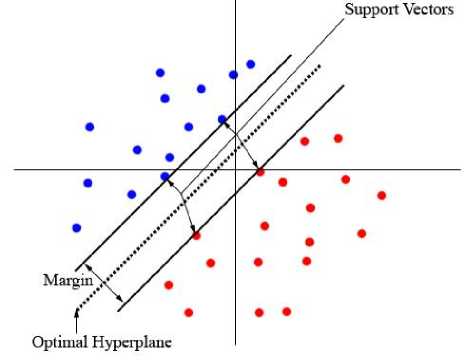
Fig. 1. The optimal Hyperplane.

A. Mathematical formulation

Consider a binary classification problem with N training points { x , , y, } , i = 1,..., N , where each input x i has D attributes and is one of two classes y i e { - 1,1 } . The data training have the following form:

{ x , , y, } where i = 1,..., N , y_t e { - 1,1 } , x , e R D       (1)

The hyperplane can be described by:

w, x , + b b = 0

where w is the norm to the hyperplane and    is the

w perpendicular distance from the hyperplane to the origin.

Finding the optimal hyperplane is equivalent to solving the following optimization problem:

•    1 t min— w w

<       2

y, ({ w , x , } + b ) >  1, i = 1,..., N

It's a primary form of quadratic problem. In order to cater for the constraints in this minimization, we need to allocate them Lagrange multipliers a and finally we have the dually form:

'       N        1

^max § a ^- ^ § ^a , , ^a j y , y j ( ^x , , x j

,=1          2., j a >0

§ a=0

By solving the equation (4), we determine the Lagrange multipliers a and the optimal hyperplan is given by:

*

w

N

§ aiУiXi i=1

*        1 *

^b =-7 w , x r + x

2 ^s

** w , x ) + b )

Where x_r and x_s are any support vectors from each class satisfying:

a _r , a s >  0, y_r =- 1, y s = 1

Solving the optimization problem requires the use of optimization quadratic algorithms such as: SMO, Trust Region, Interior Point, Active-Set, etc.

• III.    Different Variant of SVM

• A.    SVM by Sequential Minimal Optimization (SVM-SMO)

Invented by Jhon Platt [13], [14], [15] in 1998 at Microsoft research, Sequential Minimal Optimization (SMO) has been widely used for training Support Vector Machines and has been an algorithm for efficiently solving the optimization problem which arises during the training data of SVM.

To solve the quadratic problem of SVM, SMO find the solution by decomposing the quadratic problem into subproblems and solving the smallest possible optimization problem involving two Lagrange multipliers at each step.

The advantage of SMO lies in the fact that solving two Lagrange multipliers can be done analytically. Thus, numerical QP optimization is avoided entirely.

There are two components to SMO: an analytic method for solving for the two Lagrange multipliers, and a heuristic for choosing which multipliers to optimize.

In order to solve for the two Lagrange multipliers, SMO first computes the constraints on these multipliers and then solves for the constrained minimum:

The bounds L and H are given by the following:

• >    If y , ^ y j , L = max(0, O o’ld - a °^{l d} )

H = min( C , C + a ^old - a °^lld )                     (8)

• >    If y , = y j , L = max(0, a ^old + a o ^ld - C )

H = min( C , a ^old + a ^old )                        (9)

For a current solution ( a old , a°^{l d} ), the new solution ( а П™ , a jew ) is obtained by using the following update rule:

y, ( E_t - E )

new      old     j i     j a j — a j-- n

Where

Ek — f(xk)- yk n — 2( xi, xj у (x,, x,) - j, xj

E k is the error between the SVM output on the k ^th example and the true label y k .

Next we clip a new to lie within the range [L, H] i.e

L <  a new <  H , to	satisfy the constraint that 0 <  a j	< C :
1 H	si    a new >  h
a n-ew' — J L new a j	si     a new <  L si L <  a jew <  H	(12)

Finally, having solved for a new , the value of a new is given by :

a ^new — a ^old + _y._yj ( a ^old - a ^old ) (13)

The choice of Lagrange multiplier α i must violates the Karush-Kuhn-Tucker (KKT) conditions for the optimization problem and we pick a second multiplier α j and optimize the pair (α i, α j ) .

When all the Lagrange multipliers satisfy the KKT conditions (within a user-defined tolerance), the problem has been solved.

Although this algorithm is guaranteed to converge, heuristics are used to choose the pair of multipliers so as to accelerate the rate of convergence.

• B.    Least Square SVM (LS-SVM)

Proposed by Suykens and Vandewalle [16], [17], [18], Least Squares Support Vector Machines (LS-SVM) are reformulations to the standard SVMs which lead to solving linear KKT systems. LS-SVM is closely related to regularization networks and Gaussian processes but additionally emphasizes and exploits primal-dual interpretations. In LS-SVM the minimization problem is reformulating as follows:

I          N2L_ min— wlw + — Ye 2C

J      2       2" i - c                          (14)

, — 1

_ У1 (( ^w , x i ) + ^b ) ^{— 1 - e} i , c , i ^— 1,..., ^N

The reformulation corresponds to a regression interpretation with binary targets y i — ± 1. Using y ² — 1 we have:

NN   N

Z ei, — Z( ye, )2 —Z ei i—1            i —1                      i—1

N

Z{ y -[(w, xi)+b ]} i—1

The Lagrangian for this problem is:

^N w ' w + — ^ e ² 2 1:1 i

L ( w , b , e ; a ) — —

N

• ^- Z ^a i { y. (( ^w , x i )^{+ b} ) ^{- 1 + e} i } i — 1

The KKT optimality conditions are given by:

^- = O^w = V' аД12С1,1 = l....,N ow

Ц=0^Уа;У.=0, 2 = 1^

8L                  ц

—- = 0 ^ Qi = yei, 7 = -. i =

= O^ y^w^Ei'; +6) - 1+e, = 0, 1 = 1. ,.,Л^Г

After elimination of w and e k , the solution of the optimization problem can be obtained by solving the following set of linear equations:

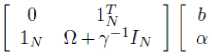
0 Y

where : Y=[y 1 ,...,y N ] ^T , 1 N =[1,...,1] ^T , α =[α 1 ,...,α N ], I N = Identity matrix, Ω= kernel function.

Finally, the classifier is found by solving a set of linear equations instead of a convex quadratic programming (QP) problem for classical SVMs. Both — and Z should be considered as hyper-parameters to tune the amount of regularization versus the sum squared error [19].

• IV. K-Nearest Neighbor

K-Nearest Neighbor (k-NN) is one of popular and simplest algorithm and it works incredibly well in practice [20], [21], [22]. K-NN is non parametric algorithm (it means that it does not make any assumptions on the underlying data distribution) and it does not use the training data points to do any generalization (no explicit training phase).

K-Nearest Neighbor uses the theory of the distance to classify a new element. It calculates the distance between the new element and the others which their classes are know. The class that appears most among the neighbors is assigned to the new element.

The choices of some parameters are very important in k-NN algorithm, these parameters are: the distance function and the parameter k which represents the number of neighbors chosen to assign the class to the new element.

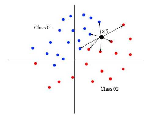
Fig. 2. The K-Nearest Neighbor.

• A.    The k-nn algorithm

The basic schema of k-NN algorithm:

• 1.    Choose a value of parameter k and the distance function.

• 2.    Given a N elements and their classes (the class of element x is c(x) ).

• 3.    For each new element y .

• 4.    Calculate the distance between y and the others elements.

• 5.    Determine the k-nearest neighbors of y .

• 6.    The new element y will be assigned to the majority class among the k-nearest neighbor.

• 7.    The class of y is c(y) .

• B.    The distances

A distance is an application which represents the length between two points. It must satisfy the following axioms:

• •    Non-negativity,

• •    Symmetry,

• •    Reflexivity,

• •    Triangle Inequality.

In the table 1, we define some distances which are very used in the literature: ( x ir , x ij : two points - x i , x j : two vectors - c xi,xj : The coefficient of Pearson correlation).

Table 1. List of some distance used in the literature.

Distances	Formulation
Euclidean	d ( xi , x j ) = Y V " j ( xi r , x jr )?
Cityblock (Manhattan)	d ( x i , xj ) = ^ " = 1 x ir - j
Cosine	V    Xir x xij d(x x ) — .________ r = 1     . J __________
	d ( x i , x j )     --------------- ---------------- nVn ( x r)? xj V" ( Xi)? \ Z—ir = 1 ir     V Z—ir = 1 jr
Correlation	d ( x i , x j ) = 1 - C xi , Xj

V. Experimentation

In this study, we analyze and evaluate the performance of different approaches of Support Vector Machines and K-nearest neighbor with several distances in the context of medical diagnosis. The evaluation has been conducted in term of: classification accuracy rate, classification time, sensitivity, specificity, positive and negative predictive values. These performance metrics are calculated by using the following equations:

Classification, accuracy:

Sensitivity: Specificity:

Positive Predictive Value :

Negative Predictive Value :

NTP+NTN^NPP+NFN NTP+NFN NTN NFP+NTN NTP NTP+NFP NTN

NTN+NFN

where :

NTP: Number of True Positives NTN: Number of True Negatives

NFP: Number of False Positives NFN: Number of False Negatives

The dataset contains informations about two diseases of urinary system which is the acute inflammation and the acute nephritis. The data was created by a medical expert as a data set to test the expert system, which will perform the presumptive diagnosis of two diseases of urinary system. The data is obtained from UCI Machine Learning Repository.

The acute inflammation of urinary bladder can be due to infection from bacteria that ascend the urethra to the bladder or for unknown reasons. This disease is characterized by: throbbing pain in the region of the bladder, occurrence of pains in the abdomen region, frequent need to urinate accompanied by a burning sensation and blood may be observed in the urine and the patient may suffer cramps after urination. If the person who suffers from this disease and does not be treated, we should expect that the illness will turn into protracted form.

The second disease is the acute nephritis of renal pelvis origin occurs considerably more often at women than at men. The first symptom of this disease is a sudden fever which exceeds sometimes 40C. The fever is accompanied by shivers and one or both-side lumbar pains which are sometimes very strong. Symptoms of acute inflammation of urinary bladder appear very often. Quite not infrequently there are nausea and vomiting and spread pains of whole abdomen.

The dataset consists of 120 instances (each instance represents a potential patient) with no missing values. It contains 9 attributes which are integer and categorical. The following table 2 describes the attributes of this database.

For each learning methods we must effectuate two essential steps: training and testing steps. In this work we have used the holdout method (which is the simplest kind of cross validation) to separate randomly the data base in two parts. Note that the k-nearest neighbor not needs a training phase.

Table 2. Attribute information of actue inflammations data set.

Attribute Description	Values of Attribute
Temperature of patient (C)	{35-42}
Occurrence of nausea	{yes,no}
Lumber pain	{yes,no}
Urine pushing	{yes,no}
Micturition pains	{yes,no}
Burning of urethra	{yes,no}
Decision : Inflammation of urinary bladder	{yes,no}
Decision : Nephritis of renal pelvis origin	{yes,no}

To validate our experimentation and the three algorithms of SVM (SMV-QP, SVM-SMO and SVM-LS), we have used several tests with different training and testing sets generated randomly by the holdout method (we made 50 tests).

The performance of k-nearest neighbor algorithm have been studies with four distances (Euclidean, Cityblock, Cosine and Correlation distance) and by using different values of " k " (between 1 and 50).

In the Fig.3, we show the classification accuracy rate obtained by (SVM-QP, SVM-SMO, SVM-LS, KNN-Euclidean Distance, KNN-Cityblock Distance, KNN-Cosine Distance and KNN-Correlation Distance).

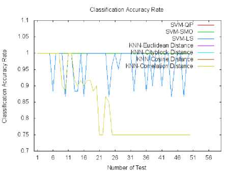
Fig. 3. The figure shows the classification accuracy rate obtained by the different approaches for all the test.

We clearly observe that the different approaches of SVM have reached a 100% classification accuracy rate. Also, for the k-NN with the four distances we record a 100% classification accuracy rate when k is between 1 and 10. When k is greater than 10 we remark a slight decrease of classification rate.

In all the various tests and by using different training and testing set in each test, SVM-QP and SVM-SMO we have obtained a 100% classification accuracy rate.

In Fig.4, we illustrate the classification time in each test and for all the different approaches.

The minimum classification time is recorded for the (SVM-QP, SVM-SMO and SVM-LS) with an advantage for SVM-QP. k-NN has the maximum classification time and this because k-NN algorithm calculates the distances between the new sample and all the sample of data set.

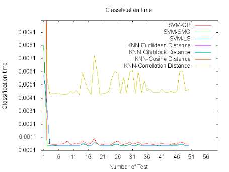
Fig. 4. The figure shows the classification time for each approaches in each tests.

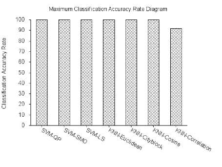
Fig. 5. The maximum classification accuracy rate between all the 50tests.

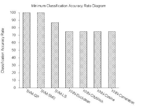
Fig. 6. The minimum classification accuracy rate between all the 50 tests.

Finally we present a summary of all results obtained followed by the sensitivity, specificity, positive and negative predictive values correspond to the maximum classification accuracy rate between the 50 tests.

VI. Conclusion

In this study, we aim to reach a high accuracy classification rate and to evaluate different approaches of

Support Vector Machines and K-nearest neighbor with different distances in acute inflammation of urinary system diagnosis. SVM-QP and SVM-SMO have achieved significant results in dealing with 100% of classification accuracy rate and a good performance in term of classification time. This experimentation showed that the proposed diagnosis SVMs could be useful for identifying the infected person.

Table 3. Sensitivity (Sens %) and specificity (Spec %), positive predictive value (Pos.P.V %) and negative predictive value (Neg.P.V %) calculated for the approaches SVMs and K-NN.

Method	Sens.	Spec.	Pos.P.V	Neg.P.V
SVM-QP	100	100	100	100
SVM-SMO	100	100	100	100
SVM-LS	100	100	100	100
KNN-Euclidean	100	100	100	100
KNN-Cityblock	100	100	100	100
KNN-Cosine	100	100	100	100
KNN-Correlation	93,33	91,11	77,78	97,61

Table 4. Summary of all Results Obtained by Svms and Knn. Average Classification Accuracy (A.C.A.R %), Average Classificaiton Time (A.C.T %), Maximum Classification Accuracy Rate (Max. %) and Minimum Classification Accuracy Rate (Min. %).

Method	A.C.A.R	A.C.T	Max.	Min.
SVM-QP	100	0,0018	100	100
SVM-SMO	100	0,0006	100	100
SVM-LS	96,80	0,0006	100	86,67
KNN-Euclidean	83,50	0,0059	100	75,00
KNN-Cityblock	84,03	0,0050	100	75,00
KNN-Cosine	89,59	0,0043	100	75,00
KNN-Correlation	84,40	0,0040	91,67	75,00