Use of an investment payback period in order to analyze project effectiveness

Many studies have been devoted to the analysis of methods of calculation of project investment payback periods and their influence on the effectiveness of investment (see e.g. [1–3]). First of all, we need to consider the undiscounted payback period PP (Payback Period). This factor is one of the most simple and widespread in world practice. The algorithm of calculation of PP depends on the regularity of the distribution of a projected investment income. If an income is distributed by year, the payback period is calculated by dividing the lump-sum cost for the size of the revenue R , i.e,

РР= K / R .

If the profit is distributed not regularly, the payback period is calculated by a direct calculation of the number of years during which an investment will be repaid with the help of a cumulative (total) income.

The indicator of a payback period is very simple in its calculations, however it has a number of disadvantages, the main one concerns the undiscounted rates on which this method is based, it does not distinguish between projects with the same amount of a cumulative income but are different in their distribution by year.

DPP (Discounted Payback Period) – this is the expected repayment period of initial discounted investments from discounted earnings. This method is similar to the previous one, but it is based on the discounted rates of investment and income. N′ is selected ( n ′) (NPV – net discounted income for n periods ′) satisfies the conditions: NPV( n ′) < 0, a NPV( n ′ + 1) > 0,then the approximation formula is used

DPP = n ‘ + NPV ( n ')/( NPV ( n ‘ + 1 ) -NPV ( n ‘ ) ) .                                            (2)

Two factors influence the discounted payback period, they are the dynamics in revenue over time and the discount rate.

Let us examine the dependence of the discounted payback period on the flow of revenue dynamics. Let us first consider a steady stream of payments (terminable annuity).

K – the amount of investments, R – steady income per period (rent income member), i – discounting.

K 1 -(1 + i) n We have — = — ---— it goes that

Ri

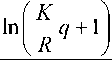
n = DPP =

- ln(1 - Ri ) ln(1 + i )

If K / R → 1/ i DPP→ ∞, i.е. if K / R ≥ 1/ i investments don’t pay off.

Now a variable flow of payments with an initial member R changes with a constant growth rate α. Then, the discounted value of an unsteady flow of payments is calculated with the help of the formula:

P = R

e q - 1

q

where q = In

1 + a

.

1 + i

The formula for DPP calculation is derived here.

DPP =

q

K, 1 + a ₁

— In--- + 1

R 1 + i

, 1 + a ln

1 + i

If α=0 (steady flow of payments) the formula (4) flows into (3).

If α= i (payments go up, but their discounted rates are steady) formula (4) according to L'Hopital's rule it flows into (1).

When α grows DPP goes down, accordingly, when α goes down DPP grows, then the condition should be able to carry out —In ⁺ a + 1 >  0 .

R 1 + i

R

Thus, when a_cr <  ( 1 + i ) e ^K - 1 investments don’t pay off (DPP^^).

For example, if K = 400, R = 100, i = 0.1, then:

a _cr = 1.1 е -°^.25 -1 = -0,143.

This example shows that when dealing with a one-time investment of 400 thousand rub. and a subsequent income stream with an initial member of the 100 thousand rub. with the pace of its change at α=0.143 – in a period, investments don’t pay off .

A great amount of a material for economic analysis is represented in the graph of the NPV (net discounted revenue) by periods of the investment cycle. Let us study three investment projects with equal one-time investments of 400 thousand rub., T =8 and various subsequent streams of income (postnume-rando). In the variant A R = 100 thousand. rub., α=0 (a constant stream of payments); variant B R =80, α=0.1 and R = 140 thousand rub., α=–0.1, i.e. income dynamics by year as follows:

А: 100, 100, 100, 100, 100, …

В: 88, 96.8, 106.5, 117.1, 128.8, …

С: 126, 113.4, 102.1, 91.9, 82.7, …

The payback period of all three projects is (4) 5 years. The graph NPV for all three projects by year is below.

As we see in Fig. 1, the curves NPV are very different.

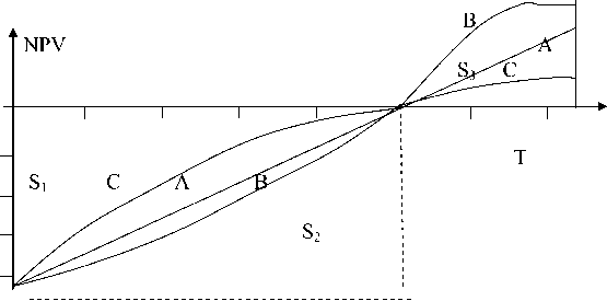
Fig. 1. Net discounted revenue for Т periods

Краткие сообщения

DPP

5 1 =- J NPV n ( t ) dt .

S 2 = DPP· K – S 1 . The best option in terms of minimizing the diversion of investment funds is one of the three considered options, which allows the recovery of spent funds more quickly. This is variant C, for which income from the beginning of the operation is higher than for the other projects. It decreases towards the end of the payback period. To quantify the differences in payback of capital investments [2] an income rise factor is introduced, which can be defined as the ratio:

p =   ⁵

5 1 + 5 2

.

The bigger the rise income factor p is, the higher the effectiveness of investments is with other things being equal. This figure has a significant disadvantage connected with the fact that it does not depend on the nature of the rise of NPV after the payback period.

In this article, we suggest a generalized indicator of the income increase, which can be defined as the integral of NPV for all periods of the investment cycle.

Т

Р = J NPV ( t ) dt .                                                                         (6)

In Fig. 1 one can see that Р = 5 3 - 5 1 , thus max p is equal to min 5 1 , that in its term gets to мах Р . So, criterion (5) is a particular case of our derived criterion (6). But the indicators PP, DPP, and criterion (5) do not take into account the influence of the income of past periods. While criterion (6) provides a comparison of investment options beyond the payback period, which removes the negative aspects that are inherent to the payback period as the indicator of effectiveness of the investment project.

There are a number of situations in which the application of a method which is based on the calculation of the payback period can be rational. In particular, this is a situation when the company’s management is more concerned with solving the problem of liquidity but are not concerned with profitability of the project – most importantly, and its investments need to be paid off as soon as possible. The method also works well in situations when investments involve a high degree of risk, therefore, the shorter the payback period is the less risky the project is. This situation is typical for industries or activities that are characterized by a fairly high probability of rapid technological change.

The suggested generalized index of the growth of an income (6) can be recommended for the analysis of the effectiveness of an investment project in all cases.

This factor takes into account the dynamics of capital investments and the dynamics of income beyond the payback period.

In Fig. 2 the graphs of NPV increase are depicted for two investment projects (project A – solid line, B – dotted line). In this case, we see that project B is more preferable than A according to criterion (6), despite the fact that its discounted payback period is larger than NPV.

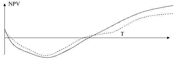
Fig. 2

This result is due to the fact that the difference of squares in the negative region of project A is greater than the difference in the positive region, so Р А < Р В .

From a technical aspect the NPV rise graph of investment project B (in comparison with project A) is provided by the following activities:

• •    execution of work that requires investments within late time frames;

• •    acquisition of an income from investments within the earliest time frames.