Using Fuzzy Models and Time Series Analysis to Predict Water Quality

Published Online April 2020 in MECS DOI: 10.5815/ijisa.2020.02.01

Water resources are vital for all living organisms on earth. Plants and animals need high quality and large quantity water to maintain basic living. However, the quality of water continues to degrade due to the ever increasing industrial and recreational effluents, which strongly threaten human health and ecosystem stability [1]. Effective measures should be taken to evaluate and model the quality of water before it is used as a drinking water resource. In the past, scientists regularly sampled the water in water quality monitoring stations, and assessed the components in the water sample in a lab. However, this process takes a long time, and thus, the detected results are not timely.

In recent decades, many machine learning techniques, like multivariate linear regression (MLR) and artificial neural network (ANN) model, have been proposed to address the problem [2-5]. A water quality dataset is a type of time series dataset that usually contains both linear and nonlinear patterns. Although machine learning techniques can save time in water quality evaluation, the prediction results of these models are not reliable, due to complex linear and nonlinear relationships hidden in the water quality dataset. Adaptive neuro-fuzzy inference systems (ANFIS) have been proven can accurately formulate the complicated nonlinear relationships hidden in the collected dataset [6]. The ANFIS model has already been used to predict water quality in many studies, and the experimental results are good. In [7], the ANFIS model shows much a higher accuracy than ANN models in the prediction of parameter dissolved oxygen (DO). Intelligence algorithms are integrated with the ANFIS model to improve the prediction performance and achieve more reliable results [8].

Although the ANFIS model can achieve good performance in water quality prediction, it has some limitations. Firstly, the size of training dataset should be not less than the number of training parameters required in the model [9]. In [7], though the ANFIS model receives higher prediction accuracy, which results in unreliable prediction. Secondly, the samples in the testing dataset should be able to gain insight from the training dataset. In some scenarios, especially when the input data has a large value range and there exist some extreme data value points, it is likely to have out-of-range errors. Unlike regular errors in the MLR or ANN models, out-ofrange errors may cause abnormal prediction results, which are extremely large or small compared to the observed values. The model can have a very large testing error even though the model can accurately predict most of the data samples. As in [10], the ANFIS model has substandard performance in the testing stage of the experiment because the limited dataset is not sufficient to build a robust and reliable model in the training stage. A stratified sampling strategy has been proposed to address the constraint of uneven distributions of datasets [11]. Lastly, an ANFIS model requires that there exists strong correlation between input and target parameters. If the correlation is weak, the ANFIS model cannot accurately formulate the hidden relationships and out-of-range errors are likely to occur in the testing stage.

Meanwhile, as the fuzzy time series (FTS) model is an accurate and reliable model to forecast time series data. It has been widely used to solve the time series dataset prediction problem [12-15]. In this paper, both ANFIS and FTS models are employed to predict water quality when the input and output parameters have weak correlations. The time series analysis method is used to preprocess the water quality dataset to figure out appropriate input parameters. A stratified sampling strategy is employed to evenly partition the whole dataset for training and testing purposes.

The organization of the remainder of the paper is as follows: Related work to review the water quality prediction model is given in Section 2. The study area, water quality parameters, and methodologies used are introduced in Section 3. In Section 4, the proposed water quality prediction system is described. Section 5 presents the experimental configuration and results. The last section concludes this paper and discusses future work.

• II.    Related Work

Generally, the quality of water resources has been manually quantized by engineers in a lab. Though this method can achieve the most accurate water quality result, it requires that professional engineers spend much time and energy with testing equipment to quantize each water quality parameter. Therefore, a linear regression model has been proposed by researchers to expedite this process [2,3]. As a water quality dataset is a type of time series data, which likely consists of a complicated linear and nonlinear relationship, the linear regression model is not reliable to address this problem, as reflected in experimental results [2].

With the emergence of ANN, various ANN models have been used to predict water quality in different scenarios. A two-layer ANN model has been applied to predict the DO concentration in the Mathura River [16], and the experimental result showed that the ANN model worked well. Four types of ANNs were investigated to predict the water temperature in [4], and the experimental result proved that all ANN models outperformed the K-nearest neighbor approach. In [17], wavelet transformation was applied to the ANN model to improve the prediction accuracy of a variety of ocean water quality parameters. A time series prediction model, namely the autoregressive integrated moving average, was integrated with the ANN model to improve the prediction performance. The experimental result showed that the hybrid model provided better accuracy than ARIMA and ANN models [5].

Although it can accurately predict water quality in some scenarios, the ANN model also has shortcomings. For example, ANN models are unable to formulate a nonlinear relationship hidden in a dataset when the input parameters are ambiguous. The ANFIS model, which can integrate the advantages of both linear and nonlinear models, outperforms the ANN model in this type of scenario. In [7], the ANFIS model was found to have better prediction results than the ANN model for DO prediction. The ANFIS model has also been applied to estimate the biochemical oxygen demand in the Surma River [18]. The testing results confirmed that the ANFIS model could accurately formulate the hidden relationship. However, building a reliable ANFIS model requires a large number of data samples, and each data sample needs to have enough strongly correlated parameters for the target parameter. As most water quality monitoring stations can only sample water monthly, the size of a water quality dataset is usually not large. When there are insufficient data samples, the ANN model tends to have better prediction performance than the ANFIS model [10,19].

The Fuzzy time series (FTS) model was first proposed by Song and Chissom in 1993 to address an enrollment prediction problem [20]. Chen improved this model by replacing complicated max-min composition operations with simplified arithmetic operations [21]. Later, the FTS model was incorporated, with trend-weighting, to improve stock price prediction accuracy [22]. The FTS model has proved to be an accurate and reliable time series data prediction model in recent years [22,23]. Several researchers have applied the FTS model to water quality prediction problems. In [13], a Heuristic Gaussian cloud transformation was integrated with an FTS model to forecast water quality. The experimental results showed that the proposed model significantly improved the prediction accuracy. However, there were only 520 water quality samples available to build the cloud, and thus, the model was not reliable or robust. As water quality dataset is typical time series data, the FTS model should be used for solving the water quality prediction problem with an adequate dataset.

In this study, fuzzy models and a time series analysis method are integrated to accurately predict water quality when the correlation between parameters is weak.

• III.    Materials and Methods

• A.    Study Area

Lake Mead is the largest reservoir in the United States in terms of water capacity and provides sustenance to nearly 20 million people, as well as a large area of farmland in Arizona, California, and Nevada. The Las Vegas Wash (LVW) is a 12-mile-long channel carrying most of the Las Vegas Valley’s excess water to Lake Mead each day. Running an average flow of 200 million gallons per day, the LVW contributes approximately 1.5% of the total flow to the lake. The flow in the wash consists of highly treated wastewater, urban runoff, shallow ground water, and storm water, where 90% of the component is wastewater effluent and industrial discharge. Therefore, it is vitally important to timely and effectively monitor and assess the wastewater quality before it discharged into Lake Mead.

Along the LVW, many organizations have built water quality monitoring stations. Six locations are selected by nearly all organizations because of their geographical advantages. These six water quality monitoring stations are labeled in Fig 1, and their geographical distribution is given.

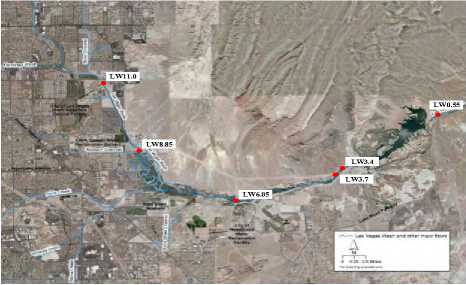
Fig.1. The geographical distribution of the six water quality monitoring stations in the Las Vegas Wash

There are three basins occupied by the Lake Mead Reservoir, with the Boulder Basin (BB) as the most western one. It lies within the boundaries of Clark County, Nevada and Mohave County, Arizona and provides drinking water resources for the people living there. The water in the BB finally joins the Lake Mead. The geographical distribution of the BB in Lake Mead is depicted in Fig. 2.

• B.    Water Quality Parameters

  In the current study, the water quality datasets collected from the LVW and BB are adopted because of high sampling frequency. LW3.4 is the key monitoring station at which if the system determines the water quality parameter exceeds the regulation limit, the water still can be treated before it is discharged into Lake Mead. The water quality datasets monitored at LW3.4 between 2005 and 2010 by LVW Coordination Committee are used to evaluate the model. There are five water quality parameters, temperature (T), pH, EC, DO, total dissolved solids (TDSs) in the collected dataset. Table 1 lists the statistical properties of these parameters. The statistical measurement of parameters, depth, pH, T, EC, and DO, in the dataset collected from the BB between 2011 and 2016 are given in Table 2. The first and second columns list the parameter label and corresponding unit, while the third column to the sixth column show the statistical properties of each parameter. The last column lists the maximum contaminant levels (MCLs) permitted by national drinking water regulations [24].

EC is used to measure the water’s ability to carry electric, and TDSs is the combination of items that are dissolved in the water. The two parameters are major indicators that quantify the quality of water. Further, DO is a necessity for all living organisms in the water. In this paper, these three parameters are selected as target parameters.

Table 1. Statistical measure of water quality parameters at LW3.4

Name	Unit	Min	Mean	Max	S. D.	MCLs
T	C	0.9	54.49	111.2	32.38	N/A
pH	unit	5.27	8.20	8.79	0.29	6.5~9.2
EC	uS/cm	1569	2463.59	2921	178.90	2000
DO	mg/L	2.42	8.28	17.95	1.80	5~14
TDSs	mg/L	1000	1580	1870	110	500

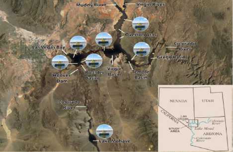
Fig.2. Location of Boulder Basin water quality monitoring station

Table 2. Statistical measure of water quality parameters at BB

Name	Unit	Min	Mean	Max	S. D.	MCLs
Depth	m	0.9	54.49	111.2	32.38	N/A
T	C	11.1	14.24	31.5	3.74	N/A
EC	uS/cm	810	927.6	1160	51.81	2000
DO	mg/L	2.30	7.63	11.30	1.17	5~14
pH	unit	6.90	7.91	9.40	0.25	6.5~9.2

• C.    Stratified Sampling

Most of the water quality monitoring stations were constructed in the past several decades, and each monitoring station may sample water every half month, one month, or one season. Meanwhile, the chemical parameters require much time and human effort to quantize. Therefore, the size of the water quality dataset and the number of parameters in each data sample tend to be small. However, the water quality dataset has completely different patterns when the water condition changes. Traditional random sampling of a small dataset could easily generate an uneven distribution of training and testing datasets. Then the data samples in the testing dataset would not be able to find clues from the training model, and thus, inaccurate predictions are likely. Stratified sampling is a sampling method widely used in classification problems to avoid uneven distribution of training and testing datasets in each category [11]. It splits the full dataset into many small strata with the same proportion of each category. This method enables the training and testing datasets to cover all of the different categories fully and evenly. In this study, the data samples are proportionally partitioned into small groups according to the quantized value of the target parameter. For each group, 75% and 25% of the data samples are selected for training and testing purposes, respectively.

• D.    Input Parameter Selection

Selecting the appropriate input parameters to build a model is fundamental to receiving accurate prediction results. It can be seen in Tables 1 and 2 that the value of each parameter has a different order of magnitude, and some have a very large range. Instead of using raw data as the input, feature scaling is adopted to normalize the value into range [0, 1]. The process can be defined as:

- x. - x ■ imin xi x - x maxmin

where x is the observed value, x and x represent the i                                  minmax minimum and maximum value of this kind of parameter, and x' is the normalized observed value.

The ANFIS model requires that the input parameters have strong correlations with the target parameters. Pearson correlation is used to calculate the correlation between parameters. Tables 3 and 4 list the correlation values between parameters in the dataset collected from the LVW and BB.

Table 3. Pearson Correlation between water quality parameters in LVW

	T	EC	PH	DO	TDS
T	1	-0.22655	0.126015	-0.4488	-0.22628
EC	-0.22655	1	0.208367	0.15019	0.999247
PH	0.126015	0.208367	1	-0.09475	0.208139
DO	-0.4488	0.15019	-0.09475	1	0.14924
TDS	-0.22628	0.999247	0.208139	0.14924	1

Table 4. Pearson Correlation between water quality parameters in BB

	Depth	T	EC	pH	DO
Depth	1	0.029396	-0.02194	-0.013	-0.05289
T	0.029396	1	0.508715	0.1725	-0.63209
EC	-0.02194	0.508715	1	-0.03386	-0.29121
pH	-0.013	0.1725	-0.03386	1	0.109696
DO	-0.05289	-0.63209	-0.29121	0.109696	1

As shown in the two tables, the correlation between parameters is very weak, except for parameters TDS and EC from the LVW. As discussed in Section 1, the ANFIS model is not applicable for cases with parameters of fairly low correlation levels. Water quality data is a type of time series data. Therefore, in this study, the timing effect of the dataset has been taken into account. When calculating the correlation between the parameters, data collected in t - 1, t - 2 and t - 3 are also taken into account. The new correlation between the parameters in the LVW and BB are given in Tables 5 and 6, respectively. The bold value in Tables 5 and 6 are the three strongest correlation value to the parameter named in each column. For example, to the parameter DO in Table 5, the value of DO in t has the top three correlation with the value of DO collected in t - 1 , t - 2 and t - 3 . Compared with Table 3, in which no qualified correlation pair exists for parameter DO, each parameter in Table 6 can find out the appropriate input for itself. The FTS and ANFIS models were used to model the prediction of water quality with the new dataset.

• E.    Fuzzy Time Series

FTS models are widely used in business and environmental forecasting. Compared to conventional time series analysis models, in which each intermediate output has only one real value, there is a fuzzy set to represent the intermediate output in the FTS model [20]. A brief definition of an FTS model is given below.

Definition 1: fuzzy time series

Let w(t )( t = ...,0,1,2,...) be the water quality dataset, which is a subset of R , the universe of discourse in which fuzzy sets f ( t )( i = 1,2,3,...) are defined. Assume that F ( t ) is a subset of f ( t )( i = 1,2,3,...), then F ( t ) is called a fuzzy time series based on w ( t )( t = ...,0,1,2,...).

In Definition 1, F ( t ) can be treated as a linguistic variable, and f ( t ) is one of the possible linguistic values of F ( t ), where f ( t ) are represented by fuzzy sets. With the changing of the universe of discourse in different times, the value of F ( t ) also changes.

Definition 2: fuzzy time series relationship

Let F ( t ) and F ( t - 1) be two fuzzy sets expressed in time series. Assuming that F ( t ) is only caused by F ( t - 1) , then the fuzzy logical relationship between the current state and the next state can be represented as F ( t ) = F ( t - 1)* R ( t , t - 1) , where * stands for an operator.

Let F ( t - 1) = A and F ( t ) = A ; the fuzzy logical relationship between the current state and the next state can be denoted as A ^ A . The steps to predict water quality with the FTS model are as follows:

Step 1: Define the universe of discourse and intervals based on the collected water quality dataset, which can be represented as: U = [min,max] . The variable min and max are the minimum and maximum values of the target parameter.

Step 2: Define the fuzzy sets according to U and fuzzify the historical data of the target parameter.

Step 3: Fuzzify the observed rules of the target parameter.

Step 4: Establish fuzzy logic relationships, and group them according to the current state of the target parameter. For example, there is a fuzzy time series, A , which has three fuzzy logic relationships: A ^ A , A ^ A , A ^ A . The fuzzy logic relationships can be grouped to: A ^A,A3,A4.

Step 5: Predict the target parameter in the testing dataset. There are two scenarios. Scenario 1: If there is only one fuzzy logic relationship: A ^ A , then the prediction value of F ( t )is A . Scenario 2: If there exist more than one fuzzy logic relationships: A ^ A , A ,—, A , the prediction value of F ( t ) is equal to the mean value of A , A ,..., A .

Table 5. Pearson Correlation of water quality parameters in LVW with time series analysis

LVW	pH(t)	EC(t-3)	EC(t-2)	EC(t-1)	EC(t)	DO(t-3)	DO(t-2)	DO(t-1)	DO(t)	TDS(t-3)	TDS(t-2)	TDS(t-1)	TDS(t)
T(t-3)	0.1045	-0.2266	-0.2326	-0.2389	-0.2456	-0.4489	-0.4463	-0.4427	-0.4392	-0.2263	-0.2326	-0.2389	-0.2456
T(t-2)	0.1095	-0.2317	-0.2265	-0.2326	-0.2388	-0.4453	-0.4489	-0.4463	-0.4426	-0.2315	-0.2262	-0.2325	-0.2388
T(t-1)	0.1164	-0.2379	-0.2316	-0.2265	-0.2325	-0.4426	-0.4452	-0.4489	-0.4463	-0.2376	-0.2314	-0.2262	-0.2325
T(t)	0.1260	-0.2442	-0.2379	-0.2316	-0.2264	-0.4386	-0.4425	-0.4452	-0.4488	-0.2440	-0.2376	-0.2314	-0.2262
EC(t-3)	0.1825	1	0.8501	0.7318	0.6310	0.1501	0.1468	0.1457	0.1454	0.9992	0.8493	0.7319	0.6307
EC(t-2)	0.1902	0.8501	1	0.8499	0.7315	0.1476	0.1503	0.1470	0.1459	0.8497	0.9992	0.8492	0.7316
EC(t-1)	0.1995	0.7318	0.8499	1	0.8497	0.1440	0.1477	0.1505	0.1472	0.7311	0.8495	0.9992	0.8490
EC(t)	0.2082	0.6310	0.7315	0.8497	1	0.1460	0.1441	0.1479	0.1507	0.6300	0.7308	0.8493	0.9992
pH(t-3)	0.8795	0.2084	0.1962	0.1850	0.1737	-0.0947	-0.0968	-0.0953	-0.0940	0.2082	0.1958	0.1846	0.1733
pH(t-2)	0.9145	0.1997	0.2084	0.1961	0.1849	-0.0950	-0.0947	-0.0968	-0.0952	0.1997	0.2081	0.1958	0.1845
pH(t-1)	0.9532	0.1903	0.1996	0.2083	0.1960	-0.0974	-0.0949	-0.0947	-0.0967	0.1902	0.1996	0.2080	0.1957
pH(t)	1	0.1825	0.1902	0.1995	0.2082	-0.0950	-0.0974	-0.0949	-0.0947	0.1826	0.1901	0.1995	0.2079
DO(t-3)	-0.0957	0.1501	0.1476	0.1440	0.1460	1	0.9584	0.9399	0.9341	0.1492	0.1468	0.1431	0.1452
DO(t-2)	-0.0974	0.1468	0.1503	0.1477	0.1441	0.9584	1	0.9584	0.9399	0.1459	0.1494	0.1469	0.1433
DO(t-1)	-0.0949	0.1457	0.1470	0.1505	0.1479	0.9399	0.9584	1	0.9584	0.1449	0.1460	0.1496	0.1471
DO(t)	-0.0947	0.1454	0.1459	0.1472	0.1507	0.9341	0.9399	0.9584	1	0.1446	0.1451	0.1462	0.1497
TDS(t-3)	0.18269	0.9992	0.8497	0.7311	0.6300	0.1492	0.1459	0.1449	0.1446	1	0.8490	0.7312	0.6301
TDS(t-2)	0.19017	0.8493	0.9992	0.8495	0.7308	0.1468	0.1494	0.1460	0.1451	0.8490	1	0.8488	0.7309
TDS(t-1)	0.19952	0.7319	0.8492	0.9992	0.8493	0.1431	0.1469	0.1496	0.1462	0.7312	0.8488	1	0.8486
TDS(t)	0.20797	0.6307	0.7316	0.8490	0.9992	0.1452	0.1433	0.1471	0.1497	0.6301	0.7309	0.8486	1

Table 6. Pearson Correlation of water quality parameters in BB with time series analysis

BBMS	T(t)	EC(t-3)	EC(t-2)	EC(t-1)	EC(t)	pH(t-3)	pH(t-2)	pH(t-1)	pH(t)	DO(t-3)	DO(t-2)	DO(t-1)	DO(t)
Depth(t)	0.0343	-0.0217	-0.0212	-0.0202	-0.0206	-0.0130	-0.0080	-0.0096	-0.0059	-0.0532	-0.0528	-0.0511	-0.0496
T(t-3)	0.9924	0.5086	0.5077	0.5072	0.5073	0.1726	0.1725	0.1725	0.1725	-0.6320	-0.6330	-0.6357	-0.6368
T(t-2)	0.9930	0.5073	0.5086	0.5078	0.5072	0.1727	0.1727	0.1725	0.1725	-0.6291	-0.6320	-0.6332	-0.6358
T(t-1)	0.9961	0.5062	0.5073	0.5086	0.5078	0.1725	0.1728	0.1727	0.1725	-0.6261	-0.6291	-0.6322	-0.6332
T(t)	1	0.5058	0.5063	0.5074	0.5087	0.1729	0.1727	0.1729	0.1729	-0.6213	-0.6262	-0.6292	-0.6322
EC(t-3)	0.5058	1	0.9964	0.9947	0.9941	-0.0337	-0.0346	-0.0351	-0.0353	-0.2910	-0.2916	-0.2929	-0.2936
EC(t-2)	0.5063	0.9964	1	0.9964	0.9947	-0.0340	-0.0337	-0.0347	-0.0352	-0.2900	-0.2911	-0.2917	-0.2931
EC(t-1)	0.5074	0.9947	0.9964	1	0.9964	-0.0343	-0.0341	-0.0338	-0.0348	-0.2891	-0.2901	-0.2912	-0.2918
EC(t)	0.5087	0.9941	0.9947	0.9964	1	-0.0341	-0.0344	-0.0342	-0.0340	-0.2876	-0.2892	-0.2903	-0.2914
pH(t-3)	0.1729	-0.0337	-0.0340	-0.0343	-0.0341	1	0.96742	0.9483	0.9350	0.1094	0.1062	0.1029	0.1015
pH(t-2)	0.1727	-0.0346	-0.0337	-0.0341	-0.0344	0.9674	1	0.9673	0.9482	0.1076	0.1091	0.1057	0.1024
pH(t-1)	0.1729	-0.0351	-0.0347	-0.0338	-0.0342	0.9483	0.9673	1	0.9673	0.1064	0.1073	0.1087	0.1054
pH(t)	0.1729	-0.0355	-0.0352	-0.0348	-0.0340	0.9350	0.9482	0.9673	1	0.1077	0.1061	0.1069	0.1084
DO(t-3)	-0.6213	-0.2910	-0.2900	-0.2891	-0.2876	0.1094	0.1076	0.1064	0.1077	1	0.9902	0.9845	0.9836
DO(t-2)	-0.6262	-0.2916	-0.2911	-0.2901	-0.2892	0.1062	0.1091	0.1073	0.1061	0.9902	1	0.9902	0.9845
DO(t-1)	-0.6292	-0.2929	-0.2917	-0.2912	-0.2903	0.1029	0.1057	0.1087	0.1069	0.9845	0.9902	1	0.9902
DO(t)	-0.6322	-0.2936	-0.2931	-0.2918	-0.2914	0.1015	0.1024	0.1054	0.1084	0.9836	0.9845	0.9902	1

Step 6: De-fuzzify. Apply the “Centroid” method to calculate the final prediction result [22].

• F.    Adaptive Neuro-Fuzzy Inference System

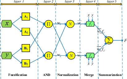
The ANFIS is a hybrid learning model, which integrates the neural network and fuzzy logic into an integrity system. The system can achieve high performance in formulating nonlinear relationships and forecasting chaotic time series. It can construct a reliable and accurate input-output mapping relationship based on the fuzzy if-then rules. The ANFIS model used in this study is generated based on the fuzzy model proposed in [25]. Given two input parameters, x and y , and one output function f , the rule set built upon the model can be expressed as follows:

where A , A , B and B represent four input membership functions for input parameters x and y . In this example, each input has two membership functions. The value of the consequent parameters a , b and c are calculated by the least square error method.

Backward Pass

Forward Pass

Fig.3. The architecture of ANFIS model with a two-input first-order Sugeno fuzzy model with two rules

The data flow in Fig. 3 illustrates the process of deriving the output from two inputs by the fuzzy reasoning mechanism and neural network strategy. The Gaussian, triangular, trapezoidal, sigmoid, spline, and generalized bell shaped input membership functions are used, and the number of each membership function corresponding to each input is configured under the constraint of the size of the available dataset.

• G.    Wavelet Transform

Wavelet Transform (WT) is widely used in the analysis of time series signals. According to the way the scale parameter is discretized, it is classified into continuous or discrete WT. As continuous WT requires a large number of data samples, discrete WT is selected as the de-noising technique in this study. Discrete WT decomposes the input signal into a mutually orthogonal set of wavelets by using a discrete set of the wavelet scales and translations. Compared to continuous WT, it requires much less computation time and is simpler to develop. Given a limited number of the highest coefficients of the discrete WT spectrum, an inverse transform can be performed with the same wavelet basis to remove the noise hidden in the true signal. The corresponding wavelet transformation can be defined as:

+ю

WT x ( a , b , / ) = — J f ( t / I      I dt      (4)

4a^m •'        I a )

where the variables n and m are integers that control the wavelet dilation and translation, a is the scale index parameter and b is the time shifting parameter (a.k.a. translation parameter). All of the points that can be represented as (a^m, na^mb) are included in the subset of the wavelet scales and translations. / ( t ) is a continuous function in both time and frequency domain called mother wavelet, and f ( t ) is the input signal or time series.

• H.    Evaluation Metrics

There are many evaluation metrics available to examine the performance of the proposed model. In this study, the mean average percentage error (MAPE), root mean square error (RMSE), and coefficient of determination (R2) are adopted to compare the performance of different models. MAPE is to represent the difference between the predicted value and true value in percentage form. RMSE is the value calculated by rooting the square of the mean of the residuals between the true value and the predicted value. R2 is an indicator to show how close the data are to the fitted regression line. The mathematical definition of each evaluation metric is given below:

n

RMSE = \ - Z (ye - Угие, )2

V n , = 1

MAPE = - ZZ | ytrue  ypred' | x 100% n -=i

n

У (У      У.)

predi       truei

R2 = 1 - -i=---------------- n

Z ( y^e, - У mean ) =1

where index i represents the position of the element in the vector, y_true is a vector holding all of the observed value, y _mean stands for the average value of vector y_true , y _pred is a vector storing all the forecasting value, and n is the size of the dataset.

• IV.    Results and Disscussion

• A.    Water Quality Dataset

  The water quality dataset collected from the LVW between 2005 and 2010, and the BB between 2011 and 2016, are used to measure and compare the performance of different models. There are 4869 and 7502 data samples available in the two water quality datasets, respectively. The observed value of parameters of EC, TDS, and DO, obtained from the water quality dataset in LVW, are given in Fig. 4. It can be seen from the figure that only parameters EC and TDS have strong correlation. Fig. 5 presents the observed value of the two parameters, EC and DO, collected at the BB water quality monitoring station. The value of EC has been divided by 1000 and 100 in the LVW and BB data, respectively, for visualization convenience. The whole dataset is split into two parts by 75% and 25% for training and testing purposes, which is the general data division percentage in data driven research experiments.

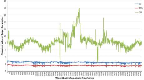
Fig.4. The observed value of five parameters in LVW between

2005 and 2010

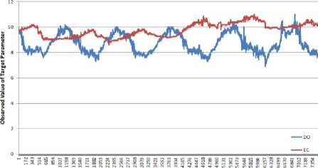
Water Quality Sample, in Time Series

Fig.5. The observed value of four parameters in BB between 2011 and 2016

• B.    Experimental Configuration

Four different kinds of models, ANN with a time-series dataset (ANN-TS), FTS, ANFIS with an original dataset, and ANFIS a with time-series analysisi dataset (ANFIS-TS) are implemented to investigate the prediction performance of each model. The ANN model built in this study is based on the model proposed in [2]. In the three-layer neural network, the input layer has three nodes and the hidden layer has four nodes. The activation function used is the linear activation function. Gradient descent is used to minimize the root mean square error between the true value and the prediction value in each iteration. The TensorFlow machine learning library is used to implement the ANN models. The FTS model is developed by the weighted FTS model proposed in [22]. The ANFIS model and wavelet transformation are developed by the MATLAB toolbox. A stratified sampling strategy is employed to split the collected dataset into the training and the testing subsets. The experimental results of the ANFIS and ANFIS-TS models are compared to verify the effectiveness of the time series analysis method in a dataset with weak correlation.

• C.    Performance Evaluation

  The experimental results of parameters EC, DO, and TDS prediction from the LVW are given in Tables 7, 8 and 9. The top three correlation coefficients of parameter EC in t include TDS in t, EC in t -1 and TDS in t -1, which are used as the input parameters to predict EC. The experimental result from Table 7 shows that the ANFIS-TS model has the best performance, which had the smallest training and testing errors, 6.73 and 4.70 measured by RMSE, respectively. Table 5 shows that the three strongest correlation inputs of parameters DO are the data itself, collected in the past three time units. In this scenario, the FTS model has a much higher prediction accuracy than the other three models, achieving 0.23 and 0.17 in RMSE in the training and testing stages, respectively. Compared to the other three models, even the most accurate one has training and testing errors of 0.37 and 0.73 in RMSE, respectively. The parameter TDS has a similar correlation pattern with parameter EC. It has a stronger correlation with the value of EC in t , EC in t -1 and TDS in t -1. The experimental results show that the ANFIS-TS model also has the best training performance, and the ANFIS has the smallest testing error, which is 0.0063, compared with 0.0064 of ANFIS-TS.

The correlation coefficients between the water quality parameters from BB are presented in Table 6. Each parameter obviously has stronger correlation with its historical record than the other parameters. This correlation pattern is similar to the correlation of parameter DO from the LVW. The aforementioned four water quality prediction models are implemented to investigate the prediction performance with the selected input and target parameters. The experimental results are listed in Tables 10 and 11. The FTS model has the smallest testing error, which could greatly reduce the prediction error. In the prediction of parameter EC from the BB dataset, the FTS model achieves the best testing performance, even though the ANFIS-TS model has a smaller training error. It shows that the FTS model is more reliable than the ANFIS-TS model in the testing stage. For parameter DO, the FTS model has the smallest error in both training and testing stages. This experimental result proves that the FTS model works better than the ANFIS and ANFIS-TS if the target parameter only has strong correlation with its historical data.

Table 7. The training and testing performance of different models for parameter EC in LVW

Models	EC
	Training			Testing
	RMSE	MAPE	R 2	RMSE	MAPE	R 2
ANN-TS	32.92	1.321	0.966	53.67	2.114	0.909
FTS	35.00	0.977	0.959	44.91	1.310	0.911
ANFIS	7.48	0.159	0.998	5.12	0.164	0.999
ANFIS-TS	6.73	0.160	0.999	4.70	0.160	0.999

Table 8. The training and testing performance of different models for parameter DO in LVW

Models	DO
	Training			Testing
	RMSE	MAPE	R2	RMSE	MAPE	R2
ANN-TS	0.68	7.290	0.856	0.90	8.018	0.746
FTS	0.23	2.015	0.987	0.17	1.909	0.960
ANFIS	1.49	11.398	0.315	1.52	11.503	0.284
ANFIS-TS	0.37	2.721	0.954	0.73	3.275	0.834

Table 9. The training and testing performance of different models for parameter TDS in LVW

Models	TDS
	Training			Testing
	RMSE	MAPE	R2	RMSE	MAPE	R2
ANN-TS	0.020	1.242	0.970	0.035	2.173	0.903
FTS	0.022	0.998	0.961	0.0279	1.334	0.916
ANFIS	0.004	0.158	0.999	0.0063	0.169	0.997
ANFIS-TS	0.003	0.162	0.999	0.0064	0.175	0.997

Table 10. The training and testing performance of different models for parameter EC in BB

Models	EC
	Training			Testing
	RMSE	MAPE	R2	RMSE	MAPE	R2
ANN-TS	11.57	1.060	0.952	11.35	1.061	0.954
FTS	4.03	0.358	0.993	4.70	0.391	0.975
ANFIS	36.99	3.089	0.510	37.85	3.163	0.488
ANFIS-TS	3.89	0.228	0.994	11.34	0.267	0.954

Table 11. The training and testing performance of different models for parameter DO in BB

Models	DO
	Training			Testing
	RMSE	MAPE	R2	RMSE	MAPE	R2
ANN-TS	0.418	4.428	0.687	0.629	6.102	0.293
FTS	0.053	0.551	0.995	0.075	0.655	0.989
ANFIS	0.406	3.623	0.705	0.408	3.655	0.702
ANFIS-TS	0.095	0.764	0.984	0.126	0.814	0.972

The predicted values of the parameters EC, DO, and TDS from the LVW using ANFIS-TS and FTS models vs. the observed values are depicted in Fig. 6. The left part is the testing result obtained by the ANFIS-TS model, and the right part is the testing result obtained by the FTS model. For parameters EC and TDS, which have strong correlation with other parameters, the experimental results from Tables 7 and 9 show that the ANFIS-TS model is a better choice in this kind of scenario. The observed value and the predicted value of the ANFIS-TS model are very close to the regression line, except for a few errors. The parameter DO only has strong correlation with itself. The training and testing data are split in a time manner. The FTS model achieved the best performance as compared to the other three models. The prediction result of the FTS model fluctuates around the observed value, which proves that this model is accurate and reliable in this scenario.

Similar to the scenario of the DO of the LVW, the DO and EC from the BB only have strong correlations with themselves. The training and testing results from Tables 10 and 11 furtherly prove that the FTS model can perform accurate prediction for this type of parameter. Fig. 7 shows that the predicted value fluctuates around the observed value except in some extreme scenarios. Compared to the ANFIS-TS model which has a few out-of-range errors, the FTS model is more accurate in this scenario.

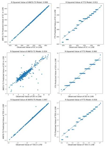
Fig.6. The coefficient of determination value of ANFIS-TS and FTS model in testing dataset of parameter EC, DO and TDS from LVW

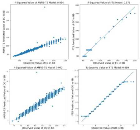
Fig.7. The coefficient of determination value of ANFIS-TS and FTS model in testing dataset of parameter EC and DO from BB

• V.    Conclusions

For getting more clear result, track initiation will be The ANFIS model can accurately formulate hidden linear and non-linear relationships in the dataset. However, The ANFIS model has strict requirements for the dataset, such as the size of the dataset and the correlation between the parameters in the dataset. If the dataset cannot meet the requirements, the prediction result is likely to be unreliable. As a water quality dataset is a kind of timeseries dataset, the time series impact must be considered, and thus, the number of input parameters of the original dataset scaled to four times. For each target parameter, the input parameter is selected based on the correlation relationship, built upon the scaled dataset.

Two water quality datasets are used to evaluate the prediction accuracy of ANN-FS, ANFIS, ANFIS-TS and FTS models. It can be seen from the experimental results that the FTS model could accurately predict the value of a target parameter when the target parameter has strong correlation with its historical record. It can be seen that the parameter DO from the LVW, and the parameters DO and EC from the BB belong to this category, with the results proving that FTS model had the best performance overall for the four models. On the other hand, when the target parameter has a strong correlation with other parameters, except itself, like parameters EC and TDS from the LVW, the ANFIS-TS model achieved better prediction accuracy over other models. This demonstrates that using the FTS and ANFIS models, integrated with time-series analysis, is an effective and reliable tool to model water quality, even when the correlation between the original parameters is weak.

Acknowledgement

The authors wish to thank the Las Vegas Wash Coordination Committee and United States Geological Survey for providing datasets for this research.