Using genetic programming techniques for inertia-free system identification tasks

Introduction. The identification of many stochastic objects is often limited to the identification of static systems. The most common pattern of the discrete-continuous process is shown in fig. 1 [1–4].

А is unknown object’s operator, x ( t ) is the vector of the object’s output variables; u ( t ) is the vector of the object’s input variables; ц ( t ) is the vector of the object’s controlled but unmeasurable input variables; X ( t ) is the vector of the object’s and controlled but unmeasurable input variables; £ ( t ) is the random action, to¹ ( t ) : i = 1,2, ..., k are the variables in the process; ( t ) is the continuous time; H ^ц , H u , H , H , H , H^to measuring devices; ц _t , u_t , x_t , to _t are measures of ц ( t ), и ( t ), x ( t ), to ( t ); h ^ц ( t ), h^u ( t ), h^x ( t ), h ^to ( t ) are the random effects.

Levels of a priori information. Let’s consider the different levels of priori information [5–7]:

• 1.    Systems with parametric uncertainty. Parametric level of priori information assumes that there is a parametric structure with unknown parameters. Iterative probabilistic procedures are used for parameter estimation. The problem of identification in the narrow sense is solved in this case;

• 2.    Systems with nonparametric uncertainty. A nonparametric level of priori information does not have the parametric structure, but it has some qualitative information about the process. For example it has uniqueness, or ambiguity of its characteristics, linearity for dynamic processes or the nature of its nonlinearity. Nonparametric statistics methods are used to solve problems of identification at this level (it is identification in a “broad” sense);

• 3.    Systems with parametric and nonparametric uncertainty. System that does not correspond to any types described above is very important from the practical point of view. For example, for individual characteristics of a multiply connected process, on the basis of physicochemical laws, energy laws, the law of mass conservation, balance relationships, parametric patterns can be derived. However, for others it is not possible.

Thus, we are in a situation where the task of identification is formulated in terms of both parametric and nonparametric priori information. Then the models are an interconnected system of parametric and non-parametric ratios.

Genetic programming. Genetic programming algorithm is based on the same optimization algorithm [8–13].

This algorithm is applied when parametric structure of process is not known, but there is a sample where (й^х,),i = 1...n , й, is the vector of the object’s input variables, xi is the object’s output variables, n is number of sample units.

Genetic programming reconstructs parametric structure, describing the process based on the available sample.

Since genetic programming is based on the optimization method (genetic algorithm), the process of finding the most optimal structure is iterative. The criterions of optimality are mean error, mean-square error, mean relative error and other characteristics that reflect structure accurateness.

The process of genetic programming is divided into the following stages [14; 15]:

• 1)    the first genetic trees are created randomly;

• 2)    receiving descendants from trees, obtaining descendants, can be performed using the following actions:

• –    Replication;

• –    Reproduction;

• –    Mutation;

• 3)    the trees that least satisfy the conditions of the optimum are destroyed;

• 4)    verification of compliance with the conditions.

It is noticeable that the genetic programming process is very similar to genetic algorithms.

Let’s describe central concepts of the genetic programming:

The concept of “genetic tree” is used as a description of the structure of an object in genetic programming. A genetic tree is a connected graph, where nodes represent actions, and finite elements (leaves) are variables (fig. 2).

We suggest the genetic tree of the following expression, as an example:

f ( x 1 , x 2 ) = x 1 *( x 2 – 7) * (2/sin( x 1 )).

The restoration of the structure from the represented tree begins with the leaves.

It is also important to describe the terms replication, reproduction and mutation.

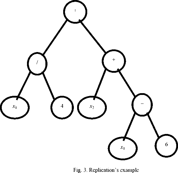
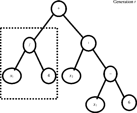
Replication is the action towards the tree that results in an exact copy of the parent tree (fig. 3).

Reproduction is receiving descendants by replacing the branches of parent trees with each other (fig. 4).

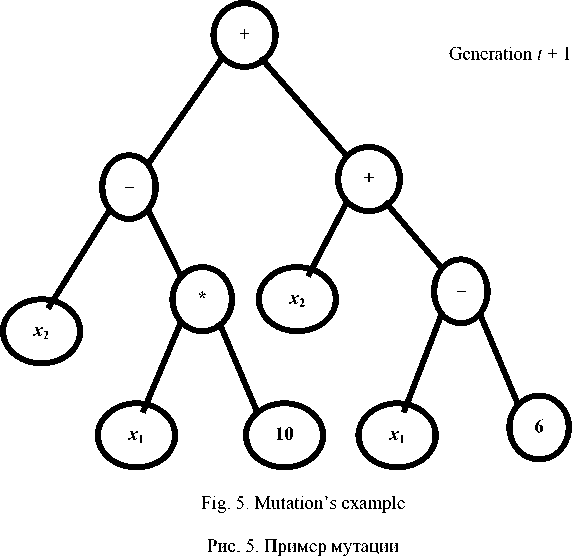
Mutation is receiving a descendant by changing the parent tree branch to randomly created one (fig. 5).

The last step in genetic programming is verification of result.

If the verification confirms to the conditions, then the researcher uses the resulting tree for object modeling.

If the conditions have not been achieved, the genetic programming process is repeated, beginning with step 2.

Computational experiment. Object modeling process is demonstrated in different conditions. In the process of computational experiments, the relationship between the dimension of the process under investigation and the speed of finding the parametric structure using genetic programming will be demonstrated.

For genetic programming, the following settings have been introduced:

• –    the number of trees = 10;

• –    prediction: average forecast error < 0.1;

• –    the maximum recovery time = 240 second.

The maximum time given for recovery is necessary to accelerate the experiment.

The structure will be restored for the following functions: f ( x ) = x 1 + x 2 + 5, x 1 e ( 0,3 ) , x ₂ e ( 0,3 ) - We will check the dependence of the time of finding the structure from the value of the training sample for this example.

The dependence of the time of finding the structure from the value of the training sample example is not observed (fig. 6). This can be explained by the fact that this algorithm more depends on “successfulness” of the original tree choice.

It is worth mentioning that during experiments the genetic algorithm was completely restored, resulting in: f ( x ) = ( x 2 + 5) + x 1 , where the restored structure does not copy the original, for example: f ( x ) = x ₁ + x ₁ + cos( x ₁) + + x 2 + 3 + sin( x 2 ), however, when x 1 e ( 0,3 ) , x 2 e ( 0,3 ) , structure is close to the original.

The structure will be restored for the following functions: fx ) = sin( x 1 )* x 1 + 6*cos( x 2 ), x 1 e ( 0,3 ) , x ₂ e ( 0,3 ) . We will check the dependence of the time of finding the structure on the value of the training sample for this example.

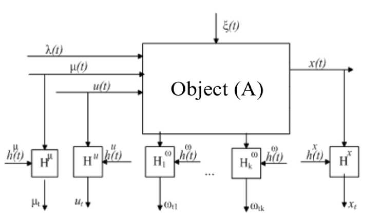
Fig. 1. Common pattern of the discrete-continuous process

Рис. 1. Общая схема исследуемого процесса

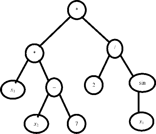
Fig. 2. Genetic tree example

Рис. 2. Пример генетического дерева

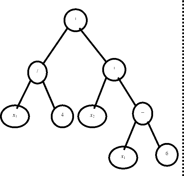
Generation t

Generation t + 1

Рис. 3. Пример репликации

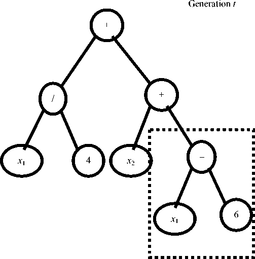
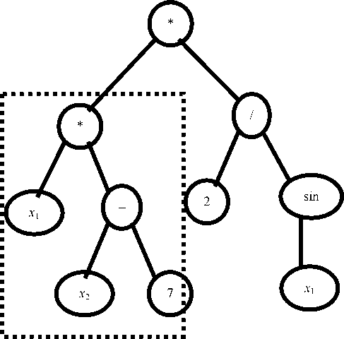
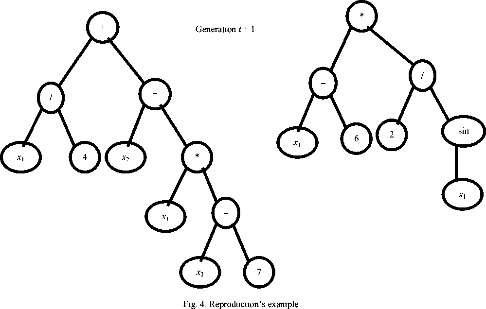
Рис. 4. Пример размножения

The dependence of the time of finding the structure on the value of the training sample example is not observed either (fig. 7).

The genetic algorithm restore the function: f ( x ) = = cos( x 2 ) + cos( x 2 ) + cos( x 2 ) + cos( x 2 ) + сos( x 2 ) + + cos( x 2 ) + ( x 1 *sin( x 1 )), but the restored structure does not copy the original, for example: f ( x ) = ((3* x 1 )/4) + + cos( x ₂)*6, but, when x 1 e ( 0,3 ) , x ₂ e ( 0,3 ) , this structure is close to the original.

When comparing fig. 6 and fig. 7, we can see that the average time to restore the structure is greater in example 2. It’s the reason to suppose that the time of modeling depends on the “complexity” of the modeling object.

Then more requires to

units (nodes and leaves) the genetic tree restore the parametric form of the original function, the more “complicated” this function is. The value of input parameters also has dependence on the “complexity”.

In the next experiment, we restore the function with 5 input variables: fx ) = x 1 + x 2 + x ₃ + x 4 + x 5 , x 1 e ( 0,3 ) , x ₂ e ( 0,3 ) . Let’s check the dependence of the modeling time on the value of the training sample.

As can be seen from fig. 8, there is no dependence of the time of finding the structure on the size of the training sample.

The genetic algorithm restores the function: f(x) = = (x5 + x3) + (x1 + (x4 + x2)), but the restored structure does not copy the original, for example: (x3 + (5 + + (((x5/4) * x3) + ((x1/(5 – x2)) * (x4 – sin(x1 + x5)))))), but, when x1 e(0,3), x2 e(0,3), this structure is close to the original.

The modeling time depends on the “complexity” of the modeling function shown in the fig. 9. You can see that in some cases the modeling process is fast. This happens in those cases when the algorithm choses the close to the desired function original tree.

As we can see in fig. 9, there is strong correlation between the modeling’s time and the value of input variables.

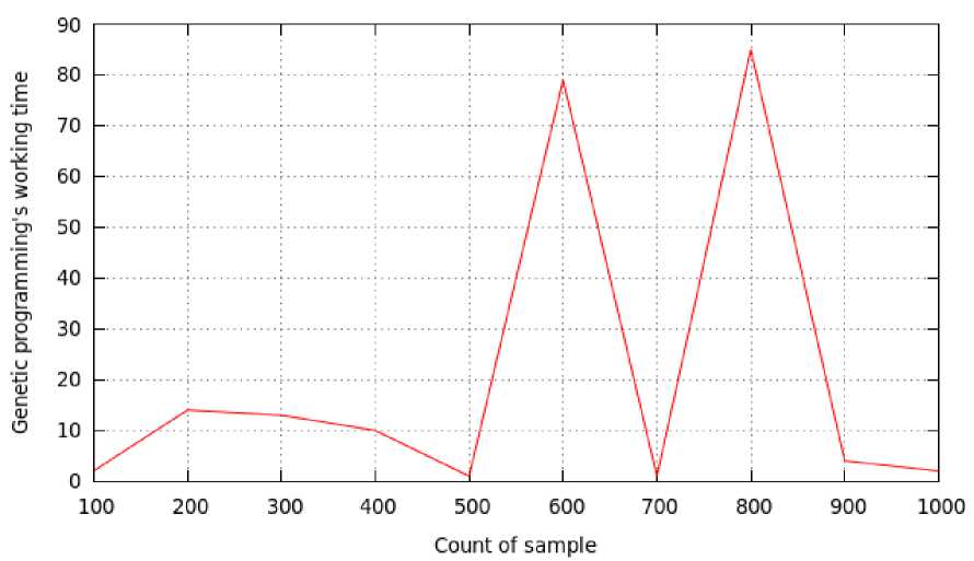
Fig. 6. Dependence of the time of finding the structure from the value of the training sample, example 1

Рис. 6. Зависимость времени нахождения структуры от величины обучающей выборки, пример 1

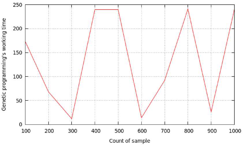
Fig. 7. Dependence of the time of finding the structure on the value of the training sample, example 2

Рис. 7. Зависимость времени нахождения структуры от величины обучающей выборки, пример 2

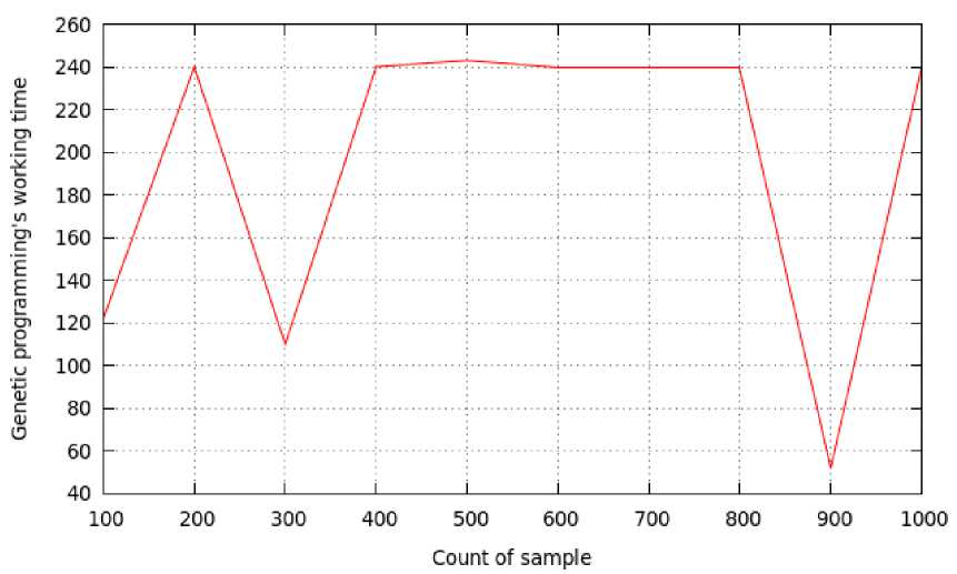
Fig. 8. Dependence of the time of finding the structure on the value of the training sample, example 3

Рис. 8. Зависимость времени нахождения структуры от величины обучающей выборки, пример 3

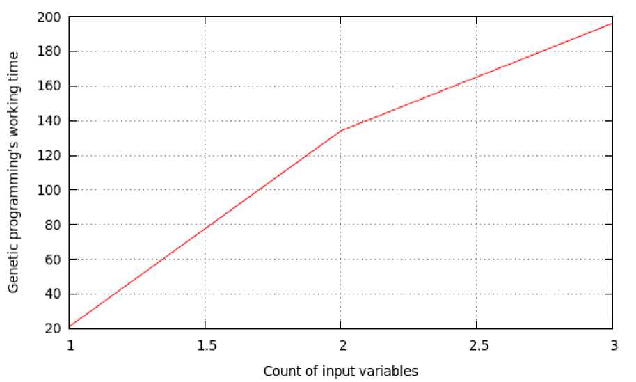
Fig. 9. Dependence of the time of finding the structure on the number of input variables, example 4

Рис. 9. Зависимость времени нахождения структуры от количества входных переменных, пример 4

Conclusion. The method of genetic programming for finding the parametric structure of the inertial-free object has been presented. It has been shown that the time of finding the parametric structure depends on train sample value. Also, the time of finding the parametric structure is dependent on the number of input variables.

Acknowledgments. The work was carried out with the financial support of the Ministry of Education and

Science of the Russian Federation during the implementation of the comprehensive project for the creation of high-tech production, contract No. 03.G25.31.0279.