Using Negative Binomial Regression Analysis to Predict Software Faults: A Study of Apache Ant

Published Online July 2012 in MECS

Software testing is one of the most important activities in software development and maintenance. It consumes considerable amount of time and resources. Because the distribution of bugs among software modules is not uniform, it would be inefficient to spend the same amount of testing time and testing effort on every module. Therefore, software defect prediction is an important technique used in software quality assurance: based on the bug history of a same or similar product, we can predict the fault-prone modules in current project. Accordingly, more testing efforts can be spent on software modules with positive predictions, which indicate the high possibilities of having bugs; and less effort can be allocated to modules with negative predictions, which indicate the low possibilities of having bugs. Considerable research has been performed in this area in recent years [1-11].

Among the many methods in predicting fault-prone software modules, negative binomial regression has been recently proposed and studied [12-15]. However, to the best of our knowledge, none of them provided detailed analysis about the performance of the prediction models, such as recall rate. Using negative binomial regression to predict software bugs is still under the stage of research, investigation, and validation. More experience and knowledge should be collected and disseminated before this method can be widely used in software industry.

In this paper, we present a case study of using class complexity metrics and product bug history to build negative binomial regression models to predict faults in software modules. Comparing with previous studies, this paper make the following contributions: (1) we present a comprehensive study of using negative binomial regression in predicting fault-prone modules and the possibility of multiple faults in a single module; (2) we compare the performance of negative binomial regression method with another popular and mature prediction meth—binary logistic regression method, in predicting fault-prone software modules; (3) we examine the performance of negative binomial regression model under two different conditions, selfassessment and forward assessment; and (4) we investigate the possibility of concept drift, which represents the changing relation between class complexity metric (explanatory variable) and software bugs (response variable), in Apache Ant.

The rest of this paper is organized as follows. Section 2 describes related work. Section 3 reviews negative binomial regression analysis. Section 4 describes the data source and data selection process. Section 5 presents the results and the analysis of this study. Conclusions are presented in Section 6.

• II.    Related Work

Using negative binomial regression analysis to predict fault-prone modules is first introduced by Ostrand et al. [15] [12]. In their studies, a negative binomial regression model was developed and used to predict the expected number of faults in every module of the next release of a system. The predictions were based on the code of the module in the current release, and fault and modification history of the module from previous releases. The predictions were applied to two large industrial systems, where they found the 20 percent of the modules with the highest predicted number of faults contained 83 percent of the faults that were actually detected. Continuous effort was spent by the same group to further investigate their prediction method [14]. In this latest study, they compared the use of three versions of the negative binomial regression model, as well as a simple lines-of-code based model, to make predictions. They also discussed the prediction differences between this study and their earlier studies. They found the best version of the prediction model was able to identify 20 percent of the system’s faulty modules, which contained nearly three quarters of the total faults.

Another study of using negative binomial regression analysis to predict fault-prone modules is reported by Janes et al. [13]. In their study, they investigated the relation between object-oriented metrics and class defects in a real-time telecommunication system. Different prediction models were built, assessed, and compared. The zero-inflated negative binomial regression model was found to be the most accurate. They further suggested applying negative binomial regression in real-world software development to predict defect-prone classes.

To summarize, comparing with other fault prediction methods, such as linear regression, binary logistic regression, and ordinary least squares, there are too little of research in predicting fault-prone modules using negative binomial regression analysis. The study reported in this paper intends to provide more experience and evidence in assessing the effectiveness of using this method to assist software quality assurance.

• III.    Method Description

Negative binomial regression analysis is a method to predicting the value of a count variable from a set of predictor variables. In this study, it is used to analyze the relations between software module attributes (complexity metrics) and the number of defects in a module. More specifically, the predicted dependent variable has a non-negative integer value, representing the number of defects in a module. The independent variables are module attributes (complexity metrics) which have continuous numerical values.

Assume Y is the dependent variable and its value is k ∈  {0, 1, 2, 3, …}, representing the corresponding module has k faults. Also assume X1, X2, …, Xn are independent variables and Pc (У = /c|x1,x2, .,^n) represents the probability that Y=k when X1=x1, X2=x2,  …, Xn=xn. Accordingly, negative binomial regression analysis can generate the following model [16]: Pc (У^Й^-^ШГ (1)

In Equation 1, r is the dispersion parameter, Г is the gamma function, and λ is the variance of Y .

Г(т) = (m - 1)!

X _ _ea + D_1X1 +b₂x₂ ⁺ .+ D_nx_n

Using negative binomial regression, we can estimate the value of dispersion parameter r and the parameters a, b 1 , b 2 , …, b n of variance λ by maximum likelihood method. Accordingly, Equation 1 can be used to predict the possibilities that certain number of bugs might exist in a module.

• IV.    Data Source

The data used in this study is obtained from online public repository PROMISE [17]. The original data is donated by Marian Jureczko, Institute of Computer Engineering, Control and Robotics, Wroclaw University of Technology [18]. Datasets of five versions of an opensource project, Apache Ant are utilized. They are Ant 1.3, Ant 1.4, Ant 1.5, Ant 1.6, and Ant 1.7. Each dataset contains the measurements of twenty static code attributes (complexity metrics) and one defect information (number of bugs) of each module (class). The detailed descriptions of these metrics can be found in CKJM web site [20]. Apache Ant is written in Java. Therefore, most of the twenty code attributes are objected-oriented class metrics, such as those defined in Chidamber and Kemerer’s metrics suite [19].

For each dataset (Ant 1.3 through Ant 1.7), we performed Spearman’s rank correlation test to determine whether each of the twenty attributes would be significant predictors in the negative binomial regression analysis. The results of the correlation tests are summarized in Table 1, where it shows the correlations between the measures of a module attributes and the number of bugs detected in that module.

Two criteria are used to select independent variables (predicting metrics): (1) In all five datasets/versions, there should be no negative correlation between the metric and the number of bugs; (2) In all five datasets/versions, there should be at least four positive correlations significant at the 0.05 level or above, between the metric and the number of bugs. Based on these two criteria, nine metrics are selected and they are bolded in Table 1. Accordingly, Equation 3 can be refined as the Equation 4, where x₁ , x₂ , …, and x₉ are the measurements of the of nine metrics: X₁ , X₂ , …, and X 9 (wmc, cbo, rfc, lcom, ce, npm, loc, amc, and max_cc). These nine metrics (independent variables) are briefly described in Table 2.

_x _ a+ +b ₁ x ₁ +b ₂ x₂ + . . .bbxX₉

Table 1: Spearman’s rank correlations between class metrics and number of bugs in that class

	Versions
Metrcis	1.3	1.4	1.5	1.6	1.7
wmc	0.377*	0.046	0.304*	0.465*	0.431*
dit	-0.031	0.156*	0.131*	-0.010	0.049
noc	0.082	0.099	0.071	0.067	0.103*
cbo	0.347*	0.168*	0.236*	0.378*	0.351*
rfc	0.426*	0.130	0.356*	0.547*	0.491*
lcom	0.316*	0.074	0.268*	0.443*	0.413*
ca	0.261*	-0.135	-0.050	0.122*	0.117*
ce	0.317*	0.365*	0.308*	0.423*	0.368*
npm	0.253*	0.027	0.270*	0.424*	0.369*
lcom3	0.064	0.129	0.018	0.037	-0.016
loc	0.401*	0.107	0.313*	0.538*	0.492*
dam	0.092	-0.033	0.119*	0.143*	0.146*
moa	0.163	0.128	0.205*	0.313*	0.337*
mfa	-0.105	0.133	0.028	-0.143*	-0.073*
cam	-0.406*	-0.001	-0.266*	-0.462*	-0.395*
ic	-0.010	0.042	0.156*	0.125*	0.128*
cbm	-0.010	0.023	0.127*	0.114*	0.130*
amc	0.203*	0.102	0.211*	0.370*	0.347*
max_cc	0.265*	0.080	0.144*	0.352*	0.380*
avg_cc	0.238*	0.052	0.102	0.277*	0.305*
*. Correlation is significant at the 0.05 level (2-tailed).

Table 2: The nine independent variables used in the prediction models

Name	Description
wmc	Number of methods defined in a class
cbo	Number of classes to which a class is coupled
rfc	Number of methods in a class plus number of remote methods directly called by methods of the class
lcom	Number of disjoint sets of methods in a class.
ce	Number of other classes that is used by a class
npm	Number of public methods defined in a class
loc	Lines of code in a class
amc	The average method size of a class
max_cc	The maximum value of McCabe’s Cyclomatic complexity of methods in a class

• V.    Results and Analysis

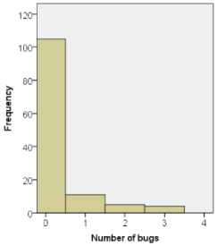
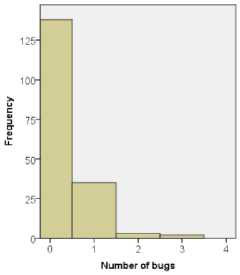
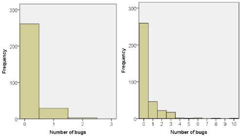
Figure 1 illustrates the distribution of the number of faults in modules of Ant version 1.3 through version 1.7, in which frequency represents the number of modules. It can be seen that in all five versions, number of bug-free modules (modules with zero bugs) accounts over 50% of all modules. Also, the frequency of classes decreases with the number of bugs. The maximum number of bugs found in one module is also different from versions to versions. For example, in version 1.5, a maximum of two bugs are found in one module, whereas in version 1.7, a maximum of ten bugs are found in one module.

• A.    Predictions description

Negative binomial regression analysis is applied on all five versions of Apache Ant. dispersion parameter r in Equation 1 and parameters a, b1, b2, …, b9 of variance λ in Equation 4 are estimated. It turns out that in all these five models (versions), dispersion parameter r is estimated having value 1. Therefore, Equation 1 can be further simplified as Equation 5, where k represents the number of faults in a module, and λ can be obtained from Equation 4.

(a)

(b)

(c)

(d)

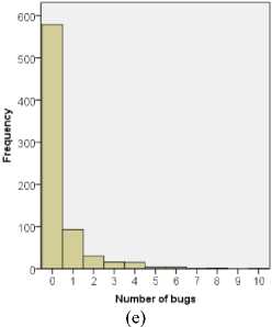
Fig 1: Distributions of bugs in modules of

(a) Ant 1.3; (b) Ant 1.4; (c) Ant 1.5; (d) Ant 1.6, and (e) Ant 1.7

^ (^Y - ^jLj         (5)

A module is said to be fault-prone if it is predicted to have at least one defect. In determining fault-prone modules, we combine the probabilities that a module has one or more bugs. Accordingly, we can derive the following two equations, where Pr( Y = 0) represents the probability that a module is bug free and Pr ( Y >  0) represents the probability that a module is fault prone (has at least one bug).

Pr (^Y = °) = 777                      (6)

Pr (Y >°)=^                (7)

In Equations 6 and 7, dependent variable Y (number of bugs in a module) has two values: positive ( Y>0 ), which indicates the module is fault-prone; and negative ( Y=0 ), which indicates the module is fault-free. The cross-analysis of predictions against observations can divide data into four categories, as shown in Table 3 ^[21]. A cut-off value (threshold) 0.5 is used in this study, which means if Pr (Y = °)value of a module is greater than 0.5 or PcYY >  °)is less than or equal to 0.5, we will consider the module fault-prone. Otherwise, we will consider the module fault-free.

Table 3: Evaluation of prediction against observation [21]

Predicted

Positive (Y>0) Negative (Y=0)

Observed	Positive (Y>0)	tp (true positive)	fn (false negative)
	Negative (Y=0)	fp (false positive)	tn (true negative)

Predication accuracy , prediction precision , and recall rate are three commonly used criteria to evaluating the prediction models. They are defined below ^[21]. Prediction accuracy describes the general prediction power of a model; prediction precision can be used to evaluate the correctness of positive signal predictions; recall rate can be used to evaluate the prediction power of positive signals. In software quality assurance, detecting fault is usually considered the most important objective. Therefore, recall rate has been used as the most important criterion in evaluating prediction models ^[22].

Prediction accuracy =	tp+tn	(8)
	tp+tn+fn+fp
P rediction precis ion =	tp tp+fp	(9)
Reca11 rate = tp		(10)

• B.    Self-assessment and forward-assessment

There are five datasets (versions) in this study. Two scenarios can be designed to build and evaluate fault prediction models: self-assessment and forward assessment. Figure 2(a) illustrates the self-assessment scenario, where one prediction model is built on each dataset and is evaluated on the same dataset. For example, the prediction model based on Version 1.3 is evaluated on Version 1.3; the prediction model based on Version 1.6 is evaluated on Version 1.6, and so on. Figure 2(b) illustrates the forward assessment scenario, where prediction models are built based on one or more datasets and evaluated on a different dataset. For example, the prediction model based on Version 1.3 is evaluated on Version 1.4; the prediction model based on Versions 1.3 and 1.4 is evaluated on Version 1.5, and so forth. We note here that similar analysis has been used in our previous study of binary logistic regression models [22].

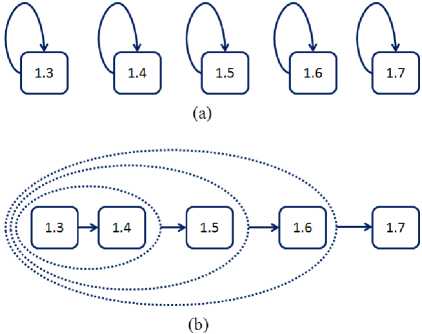
Fig 2: (a) self-assessment scenario; and (b) forward assessment scenario

Table 4 summarizes the results of self-assessment of the prediction models, which means each prediction model is evaluated on the same dataset used to build the model. It can be seen that for all five models, the prediction accuracy and prediction precision are all over 50 percent. Recall rate is relatively low for version 1.4, 8%, which means the model can predict 8% of the faulty classes. In contrast, version 1.6 has a higher recall rate, 42%, which means this model can predict 42% of the faulty classes.

Table 4: Self-assessment of negative binomial regression models

Dataset (source and evaluating)	1.3	1.4	1.5	1.6	1.7
Number of datasets	125	178	293	351	745
Prediction accuracy	87%	78%	91%	81%	81%
Prediction precision	83%	50%	100%	72%	78%
Recall rate	25%	8%	16%	42%	21%

Self-assessment is a popular method to evaluate model performance. However, in practice, prediction models are more useful if they are applied to predict faulty modules of future products. Therefore, forward assessment is used to evaluate the performance of our prediction models. Two sets of experiments are performed. The first set of experiments is to evaluate Model 1.3, which is built on source data Version 1.3 and the model is used to predict faults in Version 1.3 through Version 1.7. The results are shown in Table 5. The second set of experiments is to compare the performance of Model 1.3 through Model 1.7 on predicting faulty classes in Version 1.7. These models are built on source data Version 1.3 through Version 1.7. The results are shown in Table 6.

Table 5: Forward-assessment of the performance of Model 1.3

Source dataset	1.3	1.3	1.3	1.3	1.3
Evaluating dataset	1.3	1.4	1.5	1.6	1.7
Prediction accuracy	87%	75%	90%	78%	80%
Prediction precision	83%	33%	56%	70%	65%
Recall rate	25%	10%	44%	28%	25%

Table 6: Forward-assessment of different models

Source dataset	1.3	1.4	1.5	1.6	1.7
Evaluating dataset	1.7	1.7	1.7	1.7	1.7
Prediction accuracy	80%	79%	80%	82%	81%
Prediction precision	65%	62%	78%	66%	78%
Recall rate	25%	17%	13%	42%	21%

From Table 5, we can see that Model 1.3 is a good predictor of fault-prone classes of Versions 1.5, 1.6, and 1.7. These recall rates are higher than the recall rate of its self-assessment. Relatively speaking, the recall rate of Model 1.3 on Version 1.4 is not as good as the recall rate of the self-assessment of Model 1.3, but is better than the self-assessment of Model 1.4. From Table 6, we can see that the recall rates of the five predictions are in range 17% to 42%. Usually, self-assessment should outperform forward assessment, which has been observed in our study of binary logistic regression models [22]. However, our study of negative binominal regression of Apache Ant does not support previous observations.

Another interesting finding is that the concept drift phenomenon in not observed in our dataset. Concept drift refers to unforeseen changes in time of a concept— the dependency between class faults and complexity metrics, in our case. If the relation between explanatory variable (complexity metrics) and response variable (class faults) changes with time (versions), the prediction rules [23] should also change. In predicting fault-prone modules, if concept drift exists, we should see the aging of prediction models [24]. More specifically, if concept drift exists in our negative binominal regressions models, we should see (1) the predicting performance of Model 1.3 decreases with time (the release of new versions) in Table 5, as Version 1.4 through Version 1.7 might drift further away from Version 1.3; and (2) the predicting performance of Models 1.3 to 1.7 in Table 6 increases with versions as the source dataset is more approaching the evaluating dataset (Version 1.7). However, our analysis could not find the evidence. According, we could not confirm the existence of concept drift in our datasets.

• C.    Comparison with binary logistic regression

Following Equations 6 and 7, we can predict fault-prone modules, where modules with one or more faults are combined together and the specific number of faults in each module is ignored. This is called binary analysis, which means the predicted dependent variable only has two values, faulty or fault-free. In contrast, binary logistic regression is another commonly used technique to predict fault-prone modules [25] [26] [27] [28] [29] [30]. To evaluate the performance of our negative binomial regression models, we use the same datasets to build binary logistic regression models and compare their performance against negative binomial regression models. The results are summarized in Table 7, Table 8, and Table 9.

Table 7: Comparisons of the recall rate of two regression models (self-assessment)

Dataset   (source   and evaluating)	1.3	1.4	1.5	1.6	1.7
Number of datasets	125	178	293	351	745
Negative binomial model	25%	8%	16%	42%	21%
Binary logistic model	55%	18%	44%	42%	39%

From Table 7 through Table 9, we can see that in general, binary logistic regression models outperform negative binomial regression models in the recall rate. However, we should not be discouraged using negative binomial regression models, because their strength is predicting the number of faults in a specific module.

Table 8: Comparisons of the recall rate of two regression models: forward-assessment (1)

Source dataset	1.3	1.3	1.3	1.3	1.3
Evaluating dataset	1.3	1.4	1.5	1.6	1.7
Negative binomial model	25%	10%	44%	28%	25%
Binary logistic model	55%	23%	56%	38%	36%

Table 9: Comparisons of the recall rate of two regression models: forward-assessment (2)

Source dataset	1.3	1.4	1.5	1.6	1.7
Evaluating dataset	1.7	1.7	1.7	1.7	1.7
Negative binomial model	25%	17%	13%	42%	21%
Binary logistic model	36%	14%	33%	43%	39%

Another interesting observation in Table 8 and Table 9 is that the concept drift is not detected by the binary logistic models either. It validates the same observations using negative binomial regression models. These observations confirm no concept drift exist in our datasets.

Generally speaking, if concept drift exists in a software system, it will be harder to build long-lasting accurate prediction models; the prediction models have to be adjusted to the new releases and new bug reports. Without concept drift to worry about, negative binominal regression analysis could be relatively easily applied in real-world software development.

• D.    Multiple bug predictions

Using Equation 5, we can predict the possibilities of multiple bugs in one module. The possibilities that a module has two or more bugs, three or more bugs, and four or more bugs are calculated using the following formulas.

( ≥2)=1-∑  (  )(  )(11)

( ≥3)=1-∑  (  )(  )(12)

( ≥4)=1-∑  (  )(  )(13)

Again, cut-off value 0.5 is used in these predictions. If Pr(Ү≥n) value of a module is greater than 0.5, we will consider the module has n or more faults, where n equals 2, 3, or 4. Otherwise, we will consider the module does not have n or more faults.

In this experiment, first we examine the prediction power of Model 1.3, which is based on Version 1.3. It is used to predict the possibilities of multiple bugs in Version 1.4 through Version 1.7. The result is summarized in Table 10, where vi ^ vj indicates that vi is the source dataset and vj is the evaluating dataset. Next, we examine the prediction power of Model 1.3 through Model 1.6, which are based on Version 1.3 through Version 1.6. These models are used to predict the possibilities of multiple bugs in Version 1.7. The results are shown in Table 11, where vi ^ vj indicates that vi is the source dataset and vj is the evaluating dataset.

Table 10: Recall rate of multiple bug prediction: evaluation of Model

1.3

Number of bugs	≥ 2	≥ 3	≥ 4
1.3 ^ 1.4	0%	0%	0%
1.3 ^ 1.5	14%	0%	0%
1.3 ^ 1.6	50%	38%	20%
1.3 ^ 1.7	59%	54%	50%

Table 11: Recall rate of multiple bug prediction: evaluating on

Version 1.7

Number of bugs	≥ 2	≥ 3	≥ 4
1.3 ^ 1.7	59%	54%	50%
1.4 ^ 1.7	44%	45%	50%
1.5 ^ 1.7	77%	86%	100%
1.6 ^ 1.7	62%	55%	52%

We can see in Table 10 that Model 1.3 could not detect any classes with multiple bugs in Version 1.4. However, the performance of Model 1.3 gets better when it is used on Versions 1.5, 1.6, and 1.7: higher percentages of classes with multiple bugs are detected. Based on the information we have, we could not explain this behavior. We speculate it might be due to the increasing of number of bugs from Version 1.4 to Version 1.7. Or, it could also be due to the development differences among these versions, which are unknown to us.

In Table 11, all the models perform well on predicting classes with multiple bugs in Version 1.7. Specifically, Model 1.5 can accurately predict all the classes that have 4 or more faults. If we compare these results with bug distributions in Figure 1, the results seem encouraging. For example, in Version 1.7, 27 out of 745 (3.62%) modules have 4 or more faults, and Model 1.5 can predict all of them.

We should note here, in these predictions, although the recall rates are high, the prediction accuracy and prediction precision are usually low, which indicates the high number of false positive predictions. This accordingly might result in high cost and more effort in software testing. However, in some specific domains, such as mission critical software products, it is more important to detect faults than reducing the testing effort and testing cost. Therefore, negative binomial regression could be a powerful approach in predicting multiple bugs in a software module.

• VI. Conclusions

In this paper, we studied the performance of negative binomial regression models in predicting fault-prone software modules. The study is performed on six versions of an open-source objected-oriented project, Apache Ant. Our study shows that negative binomial regression is not as effective as binary logistic regression in predicting fault-prone modules. However, negative binomial regression is effective in predicting multiple bugs in one module, which makes it superior to binary logistic regression in this aspect.

Using negative binomial regression analysis, we found no concept drift in our dataset. Concept drift represents a changing relation between class complexity metrics and the possibility a class having bugs. This observation is further confirmed by binary logistic regression analysis.

Through this study, we wish to enrich the literature of using negative binomial regression analysis in predicting fault-prone software modules. To apply this approach in real world software quality assurance, more studies should be performed and more knowledge and experience should be collected and disseminated.

Acknowledgement

This study is partially supported by the Faculty Research Grant of Indiana University South Bend.