Using the Euler-Maruyama Method for Finding a Solution to Stochastic Financial Problems

Published Online June 2016 in MECS

Stochastic differential equation (SDE) models play a prominent role in a range of application areas, including chemistry, biology, mechanics, economics and finance [1]. These equations have become standard models for financial quantities such as asset prices, interest rate and their derivatives [2]. Ito and Stratonovich put stochastic differential equations in mathematics. Ito pioneered the theory of stochastic integral and stochastic differential equations, it use in various filed such as financial mathematics. To understand the dynamics of most SDEs and their solutions, it is important to have some knowledge of probability theory as well as some mathematical/statistical principles [3]. It is not possible to get explicit solution to many of stochastic differential equations. So, we approximate solution with numerical methods. We have based this paper around financial examples. At first, we introduce option, Brownian motion and compute discretized Brownian paths, Ito stochastic integral and stochastic differential equations. Then we survey how the Euler-Maruyama method simulate a stochastic differential equation in financial problems.

Euler method is a method for solving ordinary differential equations (ODEs) with a given initial value, it is named after Leonhard Euler who treated this method in his book (Institutionum calculi integral is published 176870). Gisiro Maruyama in 1995 showed unique answer for stochastic differential equations with Euler approximation and he proved the mean-square convergence of the Euler approximation of the Ito process without jumps, this being one of the first papers on the approximation of Ito processes [4]. Euler-Maruyama method is named after Leonhard Euler and Gisiro Maruyama.

• II.    Preliminaries

In this section, we review some of the basic concepts and definitions which are used in this paper.

• A.    Option

An option is a contract which gives the owner or holder the right to buy (call option) or sell (put option) a specified number of shares of an underlying asset at a fixed price (strike price, denoted as K ) before a specified future date or on the specified date. The time that option expires is called expiry, denoted as T . One of the most common types of options, is European option. A European option can only be exercised at its maturity. This option gives its owner the right, to buy one unit of a particular asset at a pre-set price ( K ), at some fixed future time ( T ). If the price of the asset at time T is lower than K , the option value is zero and it will not be exercised. Otherwise, if the price of the asset at time T exceeds K , the owner of the option may buy one unit of the asset at price K and immediately sell it at price S(T ), so gaining a profit of S ( T ) - K . As a result, the payoff of the European call option is:

S ( T ) - K , i/S ( T ) >  K ,

• ( S ( T ) - K ) ⁺ =            ^{,            ,             (1)}

0        , i/S ( T ) <  K .

Hence, the payoff from purchasing a European call option can be represented by the C = max( S(T ) - k ,0).

“Fig. 1,” shows payoff for a European call option with strike price $30 . Another type of option is Asian option or average option. For Asian options the payoff is determined by the average price A of the underlying asset over some pre-specified period of time as opposed to at maturity. Asian call payout is:

P (T ) = max( A (0, T ) - K ,0),            (2)

where A denote the average, and K the strike price. The average A may be shown in many ways. For the case of discrete monitoring with monitoring at time t ,..., t , the average is:

N

A (0, T ) = - E S (O-            (3)

N i = 1

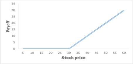
Fig.1. Payoff for European call option with strike price $30 .

• B.    Brownian motion

A Brownian motion, or Wiener process, over[0, T ] is a random variable W ( t ) that depends continuously on t e [0, T ] and satisfies the following conditions:

• 1.    W (0) = 0, With probability 1.

• 2.    For 0 <  V <  t <  T the random variable given by the increment W(t ) - W ( v ) is normally distributed N (0, t - v ) and W ( t ) - W ( v )~ 41 - v N (0,1) where N (0,1) denote normally distributed random variable with zero mean and unit variance.

• 3.  For    0 <  V < t < u < s <  T the increments

W ( t ) - W ( v ) and W ( s ) - W ( u ) are independent.

We consider discretized Brownian motion for computational purposes, where W ( t ) is specified at discrete t values. We set St = T / N (for some positive integer N ). W . Denote W ( t ) with t. = j S t . We have W = 0 with probability 1 from condition 1, from conditions 2 and 3:

W j = W j - 1 + dW j , j = 1,..., N ,            (4)

where each dW is an independent random variable of the form V S tN (0,1) [1]. MATLAB 1 [1] performs one simulation of discretized Brownian motion over [0,1] with N = 400 , and produce “Fig. 2”. Now, we simulate the stochastic function

( t + ¹ W ( t ))

u (W ( t )) = e ²                     (5)

along 2000 discretized Brownian paths over [0,1] with N = 400 . Equation (5) has the form of the answer of linear stochastic differential equations. “Fig. 3,” show average of u ( W ( t )) over 2000 discretized Brownian paths. The average of u ( W ( t )) is plotted with a solid green line. 5 individual paths are plotted with a dashed red line.

%Brownian path simulation

% vectorized randn('state', 100)

T = 1; N = 400; dt = T/N;

dW = sqrt(dt)*randn(1,N);

W = cumsum(dW);

plot([0:dt:T],[0,W],'r-')

xlabel('t','FontSize',12)

ylabel('W(t)','FontSize',12 ,'Rotation',0)

MATLAB 1. Simulation of Brownian path.

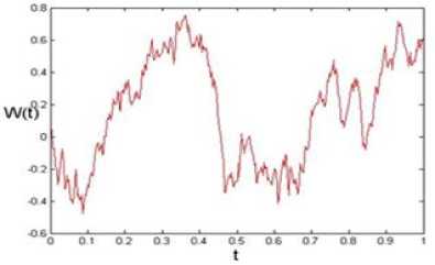
Fig.2. Simulation of discretized Brownian path over[0,1] with N=400.

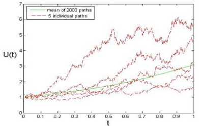
Fig.3. u ( W ( t )) averaged over 2000 discretized Brownian paths along 5 individual paths

In “Fig. 3,” the maximum discrepancy between the 9t sample average and the expected value of u(W(t)) (e 8 ) over all point t is 0.0177.

• C.    Ito integral

Let 0 = t₀ <  t_x <  ... <  t_N_ _T<  t_N = T be a grid of points on the interval[0, T ] , The Ito integral is the limit:

T                    N -1

f h ( t ) dW ( t ) = lim£ h(t j^ (W(t_j+l) - W ( j)      (6)

0                 5 t ^G^""

J =^G

• D.    Ito formula

If Y = f (t, X), then dY = f (t, x ) dt + d, (t, x ) +1 df (t, X) dxdx.   (7)

Where dxdx term is interpreted as follows:

dtdt = G, dtdW = dWdt = G,            (8)

dW_tdW_t = G.

• III.    Stochastic Differential Equations

Stochastic differential equation (SDE) is a differential equation in which some of the terms and its solution are stochastic processes [5]. SDEs are important in filtering problems, stochastic approaches to deterministic boundary value problems, optimal stopping, stochastic control, and financial mathematics [6]. A general form for a stochastic differential equation is:

dX ( t ) = f ( X ( t )) dt + g ( X ( t )) dW ( t ),

X (G) = X g ,                             (9)

G <  t <  T .

Where W denote a Brownian motion and f and g are given functions. A solution is a stochastic process, which can be interpreted as integral equation [7]:

X ( t ) = X G + Г f ( X ( 5 )) ds + Г g ( X ( s )) dW ( s ), 00       (10)

G <  t <  T .

The second integral is Ito integral. If g = G and X _o is constant, (10) reduces to the ordinary differential equation:

— = f ( X ( t )), X (G) = X G .           (11)

dt

To better understand the difference between (9) and (11) we suppose that a person has two possible investments:

• 1.    A risky investment e.g. a stock, where the price P ( t ) per unit at time t satisfies a stochastic differential equation:

• 2.    A safe investment e.g. a bond, where the price P ( t ) per unit at time t grows exponentially:

^p 1 = ( a + a ." noise ") P .          (12)

dt                         ¹

Where a >  G and a E R are constants.

dP

—2 = bP dt        2 , where b is a constant, G < b < a [8].

Equation (12) is stochastic differential equation, we don’t know the “noise” behavior. An SDE is an important model in science and engineering when noise affects behavior. For example, SDEs can model the rapidly fluctuating prices of the stock market [9]. But in (13) we don’t have the “noise” and (13) is ordinary differential equation. . The well- known Black–Scholes model of the asset price is described by the linear SDE [10]:

dX ( t ) = ^ X ( t ) dt + ^X (t ) dW (t ), X (G) = X g ,

where Ц and a are real constants. This stochastic differential equation arises, for example, as an asset pricing model in financial mathematics. The general solution of a linear stochastic differential equation can be found explicitly [11].The solution of the (14) is geometric Brownian motion [12]:

^{X (} t ) = ^X G ^exp⁽( ^ ^- -O t ⁺ a W^(t )).       (15)

Geometric Brownian Motion is nonnegative, it provides for a more realistic model of stock prices. Also, the Geometric Brownian Motion model considers the ratio of stock prices to have the same normal distribution. [13]. An alternative to the stock price model (14) is the mean reverting square root process [14]:

dS_t = a(b - S_t ) dt + c^SdW, ,       (16)

where a, b and c are constant. To check solution (15) for (14) [2], write

X = f (t , Y ) = X o e ,               (17)

where Y = (^ -1 a2)t + aW,. By the (9), dX =X eYdY+1 eYdYdY.

where dY = (µ- σ2)dt+σdW . By the (10), dYdY =σ2dt.(19)

As a result dX = X eY (µ- 1σ2)dt+X eYσdW + 1σ2X eYdt 0                                  0t0

=X eYµdt+X eYσdW(20)

= µ Xdt + σ XdW .

We use Monte Carlo simulation for linear stochastic differential equation at following example.

Example 1. Suppose following process for the stock price S :

dS = 0.16 Sdt + 0.32 SdW ,            (21)

where the stock pays no dividends, has a volatility of 32% per annum, the expected return from a stock is 16% per annum with continuous compounding and the initial stock price is $100 (S = 100 ). According to Wiener process, dW is ε δt where ε N(0,1) . Let  ΔS is the increase in the stock price in the next small interval of time. So,

Δ S = 0.16 S Δ t + 0.32 S ε Δ t .         (22)

Consider a time interval of one week or 1/52 of a year. So,

Δ S = 0.00307 S + 0.04434 S ε .         (23)

Table 1. Monte Carlo simulation of stock price where µ = 0.16 and σ = 0.32 during 1-week periods over fifteen weeks.

Stock price (at start of period)	Random sample ( ε )	Change in stock price during period
100	-0.66	-2.62
97.38	-0.46	-1.69
95.69	0.28	1.48
97.17	0.27	1.46
98.63	0.84	3.98
102.61	0.65	3.27
105.88	0.95	4.78
110.66	0.52	2.89
113.55	0.86	4.68
118.23	-0.71	-3.36
114.87	-0.44	-1.89
112.98	-0.24	-0.85
112.13	0.91	4.87
117	1.58	8.55
125.55	0.54	3.39
128.94	0.78	4.85

To produce a random sample ε from a standard normal distribution in Excel, we use NORMSINV ( RAND ()) [15]. We use Monte Carlo simulation of stock price over fifteen weeks for this example in Table 1. So, the random sample from the distribution of stock prices at the end of 15 ^th week is 128.94.

• IV.    Euler-Maruyama Method

There is a stochastic analog of Euler’s method which is known as the Euler-Maruyama method [6]. Euler-Maruyama method is constructed within the Ito integral framework [7]. To apply Euler-Maruyama method to (9) over[0, T ] , we first divide the interval. Let Δ t = T / L (for some positive integer L ) and τ = j Δ t ( j = 0,..., L ). Our numerical approximation to X ( τ ) will be denoted X . The Euler-Maruyama method takes the form [1]:

X j = X j - 1 + f ( X j - 1 ) Δ t + g ( X j - 1 )( W ( τ j ) - W ( τ j - 1 )), j = 1,..., L .

Now we want to obtain (24). Setting t = τ and t = τ in (10), we obtain:

X ( τj ) = X 0+ ∫ ^{τ j}f ( X ( s )) ds + ∫ ^{τ j}g ( X ( s )) dW ( s ). (25)

X ( τj -1 ) = X 0+ ^{τ j -1} f ( X ( s )) ds + ^{τ j -1} g ( X ( s )) dW ( s ).(26) 00

We subtract these equations ((25) and (26)):

X ( τ j ) = X ( τ j - 1 ) + ^{τ j}f ( X ( s )) ds + ^{τ j}g ( X ( s )) dW ( s ). (27) ^τ j - 1                             ^τ j - 1

For the first integral in (27) we can use the conventional deterministic quarture approximation and for second integral we use Ito formula [7]:

^{τ j} f ( X ( s )) ds ≈ ( τ j - τ j - 1 ) f ( X j - 1 ) =∆ tf ( X j - 1 ).    (28)

^τ j - 1

^{τ j} g ( X ( s )) dW ( s ) ≈ g ( X j - 1 )( W ( τ j ) - W ( τ j - 1 )).    (29)

^τ j - 1

Setting (29) and (28) in (27) gives us Euler-Maruyama formula (24).The Euler-Maruyama method has strong order of convergence ½ and weak order of convergence 1 [16]. Now, we use this method for approximating stochastic differential equations in financial problems.

Example 2. Suppose following process for the stock price:

dS = 0.16 Sdt + 0.30 SdW , S = 100.

S is the stock price at a particular time and W is Brownian motion. The exact solution to this equation is:

S, = 100exp(0.115 t + 0.30W, ).          (31)

We have a discretized Brownian path over [0,1] with S t = 2 - 8 . The solution (31) is plotted with magenta line in Fig 4. We apply Euler-Maruyama method to (30) using a step size A t = RSt with R = 32 , that is plotted as green asterisks connected with dashed lines in “Fig. 4”. The discrepancy between the exact solution (31) and Euler-Maruyama approximation at the endpoint t = T = 1 , was found to be 3.8741. Using smaller R values of 8 ( R = 8 ), shown in “Fig. 5,” (see MATLAB 2), produced endpoint errors of 0.5084. So, the endpoint errors decreased with smaller R. For better conclusion we use values of 2 ( R = 2), shown in “Fig. 6”.

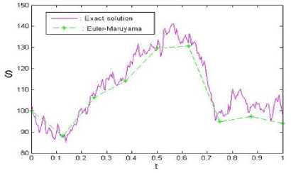
Fig.4. Exact solution and the solution based on Euler-Maruyama

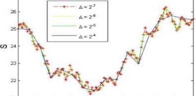
Example 3. We apply Euler-Maruyama method to a square-root asset pricing model with д = 0.09, C T = 0.6 and S_o = 25 :

We approximate this stochastic differential equation (32), for a single path but with different step sizes ( 2 ^{- 4} ,2 ^{- 5} ,2 ^{- 6} and 2 ⁷ ) [14] are shown in “Fig. 7”. According to the Example 1, we conclude that the approximation with the smallest A t is the best approximation. So, the red asterisks connected with dashed line is the best approximation.

21o    0.1    0.2    0.3   0.4 O.S 0.0   0.7    0.9   0.9

t

Fig.7. Euler-Maruyama approximation to a square-root asset pricing model with different step sizes.

approximation with step size

A t = R S t , R = 32 .

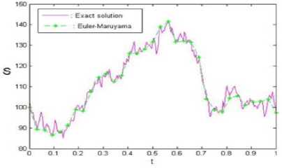
Fig.5. Exact solution and the solution based on Euler-Maruyama

A t = R S t , R = 8 .

approximation with step size

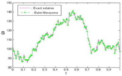
Fig.6. Exact solution and the solution based on Euler-Maruyama approximation with step size At = RSt , R = 2 .

• V.    The Approximation Payoff for A European Call Option

Let f (t, S(t))  represent the value of a European call option on stock S . Let S follow the equation

dS = Srdt + ScdW.         (33)

We want to compare Euler-Maruyama method and true solution of the payoff at the initial time. We compute the true solution and Euler-Maruyama approximation along 2000 discretized Brownian paths for different initial values, ranging from 70 to 95. The strike price K set at 83, the interest rate at 10.9%, the time T at 0.2 years and C = 0.1195 (volatility). Look at “Fig. 8”, it resembles the call payoff graph shown in “Fig. 1”. The black line represents the true solution and the x-green line represents the Euler-Maruyama approximation. The graph’s curve in “Fig. 8,” begins to rise before the strike price ( K = 83 ), that differs from the previously shown payoff graph in “Fig. 1”. This difference can be explain by the fact that graph in “Fig. 8,” is for the expected value of the payoff at the initial time, while the previously shown payoff graph was drawn at the expiration date [13].

% Euler-Maruyama method on linear SDE Stock Price.

%SDE is dS= mu*S dt + sigma*S dW, S(0) = Szero, %where mu =0.16, sigma =0.3 and Szero = 100.

%Discretized Brownian path over [0,1] has dt = 2^(-8).

%Euler-Maruyama uses timestep R*dt.

randn('state',100)

mu = 0.16; sigma= 0.3; Szero = 100;

T = 1; N = 2^8; dt = 1/N;

dW = sqrt(dt)*randn(1,N);

W = cumsum(dW);

Strue = Szero*exp((mu-0.5*sigma^2)*([dt:dt:T])+sigma*W);

plot([0:dt:T],[Szero,Strue],'m-'), hold on

R =8; Dt = R*dt; L = N/R;

Xem = zeros(1,L);

Xtemp = Szero;

linetypes={'b-','g--*'};

for j = 1:L

Winc = sum(dW(R*(j-1)+1:R*j));

Xtemp = Xtemp + Dt*mu*Xtemp + sigma*Xtemp*Winc;

Xem(j) = Xtemp;

end plot([0:Dt:T],[Szero,Xem],'g--*'), hold off legend(': Exact solution',': Euler-Maruyama')

xlabel('t','FontSize',12)

ylabel('S','FontSize',12,'Rotation',0,'HorizontalAlignment','right')

emerr = abs(Xem(end)-Strue(end))

MATLAB 2. Exact solution and the solution based on Euler-Maruyama method on linear SDE stock price.

%Euler-Maruyama method on stochastic volatility SDE asset price.

% SDE is dS(1) = mu*S(1) dt + S(2)*sqrt(S(1)) dW(1), S(1)_0 = Szero(1)

%     dS(2) = 1/2*(sigma_0- S(2)) dt + 2*sqrt(S(2)) dW(2), S(2)_0 = sigma_0

% S(1) is the asset price, S(2) represents the volatility

% European Option Price

% Vectorized across samples clf randn('state',1)

T = 1; N = 2^10; Delta = T/N; M = 1e+4;

mu = 0.16; Szero = 100; sigma_zero = 0.3; r = 0.05;

Xem1 = Szero*ones(M,1);

Xem2 = sigma_zero*ones(M,1);

for j = 1:N

Winc1 = sqrt(Delta)*randn(M,1);

Winc2 = sqrt(Delta)*randn(M,1);

Xem1 = abs(Xem1 + Delta*mu*Xem1 + sqrt(Xem1).*Xem2.*Winc1);

Xem2 = abs(Xem2 + Delta*1/2*(sigma_zero - Xem2) + 2*sqrt(Xem2).*Winc2);

end

Price = exp(-r)*mean(max(0,Xem1-1))

MATLAB 3. Estimating the value of European call option to buy the asset at the future time T (using Euler-Maruyama method).

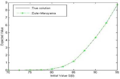
Fig.8. Euler-Maruyama approximated payoff for a European call option.

Example 4. Look at the pair of following stochastic differential equations, the first equation is the asset price model, with asset variance S ² , following second equation:

for 0 < t < 1 . The Brownian paths Wt 1 and Wt2 are independent. We setp = 0.16, SJ = 100 andS2 =

we approximate e E[max(0, St -1)] for equation (34), where S1t is the average of S1 over 0≤t ≤1, this corresponds to pricing an Asian option. MATLAB 4 produce 102.2217 (value of Asian option to buy asset at future time T ). If we exercise this option, we gain a profit of 2.2217.

% Euler-Maruyama method on stochastic volatility SDE asset price.

% SDE is dS(1) = mu*S(1) dt + S(2)*sqrt(S(1)) dW(1), S(1)_0 = Szero(1)

%     dS(2) = 1/2*(sigma_0-S(2)) dt +2*sqrt(S(2)) dW(2), S(2)_0 = sigma_0

% S(2) is the asset price, S(2) represents the volatility

% Asian Option Price

% Vectorized across samples clf randn('state',1)

T = 1; N = 2^10; Delta = T/N; M = 1e+4;

mu=0.16; Szero = 100; sigma_zero = 0.3; r = 0.05;

Xem1 = Szero*ones(M,1);

Xem2 = sigma_zero*ones(M,1);

Ssum = Xem1;

for j = 1:N

Winc1 = sqrt(Delta)*randn(M,1);

Winc2 = sqrt(Delta)*randn(M,1);

Xem1 = abs(Xem1 + Delta*mu*Xem1 + sqrt(Xem1).*Xem2.*Winc1);

Xem2 =abs(Xem2 + Delta*1/2*(sigma_zero - Xem2)+2*sqrt(Xem2).*Winc2);

Ssum = Ssum + Xem1;

end

Smean = Ssum/(N+1);

Price = exp(-r)*mean(max(0,Smean-1))

MATLAB 4. Estimating the value of Asian call option to buy the asset at the future time T (using Euler-Maruyama method).

• VI.    Conclusion

In this paper, we surveyed the applications of stochastic differential equations and Euler-Maruyama method for some financial problems. We found out the endpoint errors decreased with smaller delta ( ∆t ) for linear stochastic differential equation (the process for the stock price). Besides, we approximated square-root asset price model with different step sizes, because the solution to this equation is not explicit. Moreover, we estimated the value of European call option to buy the asset at the future time T , and we applied it for Asian option.