Utilizing Neural Networks for Stocks Prices Prediction in Stocks Markets

Published Online June 2020 in MECS

Prediction of stock market data is a crucial issue for stock traders. Stock market data have a highly dynamic property due to a conflicting extent of influential factors. The issue has been approached for business interests by observing market forces, making assumptions and recognizing historical data. Increased attention, from academia in the field of predictions, has driven to development of technical and statistical models. In contrast to conventional methodologies practiced by traders, technical methods are confined and restricted to observations of historical data. One of the most recently examined technical methods is Artificial Neural

Networks (ANN). Originating from neural networks, ANNs are mathematical structures originally designed to mimic architecture, fault-tolerance, and learning capability of neural networks existing in the human brain. ANNs have been successfully applied for prediction in the fields related to medicine, engineering and physics. The methods have been suggested for modeling financial time series due to the capability of mapping nonlinear connections as proposed for stock market data. The performance of ANNs has been compared to statistical approaches, representing significantly improved results for increasing complexity in time series. Further factors affecting the performance of ANNs are the choice of architecture, input data, and quantity of data.

In the current model, technical information of stock such was used as Open-close-High-low prices and volume of stock as training input vector of Artificial Neural Network and make the predict price function in many variable not one variable the time[16,17,25] . Also, it divided the training vector to many sets; each set was used to train an independent neural and all output of each neural formed a training set the head neural network which give the output of over All system. The first level of neural networks can train in parallel to reduce overall time of training of neural network. For the concept of the current research, it was tried to predict the price of the stock in the short term future with less Mean Square Error and fastest training time of Neural Network. The main objective was to maximize the profit by trying to increase the capital.

Through the years, the economists investigated many different methods to try and find an optimal way to predict the movement of a stock. Some of them are Japanese candlesticks [1, 15], Monte Carlo Models [2], Binomial Models [3]. However instead of using those traditional methods, the problem of predicting stock prices using machine learning techniques [9] and specifically Artificial Neural Networks was approached

• [4] . Then, it was tried to come up with an optimal trading strategy to maximize the potential profit. The main idea was to model a stock trading day using historical information of the stock, the stock price after one day was tried to be predicted. Also, it was tried to train to and test the current model on historical stock data collected during the period of 2007 to 2017 from The Egyptian stock market.

The paper in hand is organized as follows: literature review in the second section. The third section introduces the proposed back propagation research method for prediction of stock market. The fourth section deals with an illustration for simulation results of all developed controllers. And the last section includes the concluding remarks.

II.    Literature Review

Trifonov conducted a study on the architecture of a neural network which used four different technical indicators [6]. For UTOMO, improving optimization in stock price predictions can be done using a gradientbased back propagation neural network approach. Using this gradient descent in BPNN method [5]. Lin, proposed a kind of neural network which is called TreNet, a novel end-to end hybrid neural network. [7].

Hiransha presented a paper, in which there were four types of deep learning architectures, Multilayer Perceptron (MLP), Recurrent Neural Networks (RNN), Long Short-Term Memory (LSTM) and Convolutional Neural Network (CNN) [8]. Chen1 (2018), proposed a deep learning method based on Convolutional Neural Network to predict the stock price movement of Chinese stock market [18].

III.    Research Method

• A.    Backpropagation Neural Network

  The demonstration of the limitations of single-layer neural networks was a significant factor in the decline of interest in neural networks in the 1970s. The independent discovery by several researchers and widespread dissemination of an effective general method of training a multilayer neural network had a major role in the reemergence of neural networks as a tool for solving a wide variety of problems [14, 24].This training method, known as backpropagation of errors or the generalized delta rule shall be discussed. It is simply a gradient descent method to minimize the total squared error of the output computed by the net [10]. A multilayer neural network with one layer of hidden units (the Z units) is shown in Figure 1.

The output units (the Y units) and the hidden units also may have biases (as shown in Figure 1. The bias on a typical output unit Yk is denoted by W0k.The bias on a typical hidden unit Zy is denoted V0j. These bias terms act like weights on connections from units whose output is always 1. These units are shown in Figure 1, but are usually not displayed explicitly. Only the direction of information flow for the feedforward phase of operation is shown. During the back propagation phase of learning, signals are sent in the reverse direction [11].

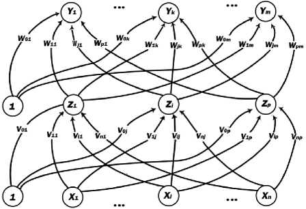
Fig.1. Multilayer neural network with one layer of hidden units

Training a network by backpropagation involves three stages: the feedforward of the input training pattern, the backpropagation of the associated error, and the adjustment of the weights [13].

During feedforward, each input unit Xi receives an input signal and broadcasts this signal to the each of the hidden units Z 1 ,...,Z p . Then each hidden unit computes its activation and sends its signal z to each output unit. Each output unit Y d computes its activation y k to form the response of the net for the given input pattern. During training, each output unit compares its computed activation Y K with its target value t k to determine the associated error for the pattern with the unit [11].Based on this error, the factor δ k (k = 1...m) is computed δ k is used to distribute the error at output unit Y_k back to all units in the previous layer: the hidden units that are connected to Y d . It is also used, later, to update the weights between the output and the hidden layer. In a similar manner, the factor δ j (j = 1...p) is ᴄcomputed for each hidden unit Z j . It is not necessary to propagate the error back to the input layer, but δ j is used to update the weights between the hidden layer and the input layer [11].

After all of the δ factors have been determined, the weights for all layers are adjusted simultaneously. The adjustment to the weight W jk (from hidden unit Z j to output unit Y k ) is based on the factor δ k and the activation Z j of the hidden unit Z j . The adjustment to the weight V ij (from input unit X i to hidden unit Z j ) is based on the factor δ j and the activation X i of the input unit [11].

• B.    The new proposed system

The new system has three main steps: data preprocessing, separating the training data set into many parts, training the neural network with each separate part.

• B.1    The Preprocessing of Data

The training vectors which consist of Open-close-High-Low-Volume are on drastically different scales. The volume had a very large value, but the price had a small value that makes the volume a factor influencing behavior of the neural network.

According to Guoqiang Zhang, B. Eddy Patuwo, Michael Y. Hu [12], data normalization is performed before the training process begins due to the fact that non-linear activation functions tend to squash the output of a node either in (0, 1) or (-1, 1). As a result, a way is needed to transfer the output of the neural network back to the original data range. Even in the case a linear output function, is used, it is also stated that normalizing the inputs as well as the outputs has many advantages. Some of them avoid computational problems, so all data input must be normalized from 0 to 1 by using Max-Min normalization equation [19-23].

,т     ..   . .         data—min value

Normalized data = max value — min value

• B.2    Separate data

  The historical data of the stock, which is 7 years from 2007 to 2014, used in training the neural network, will be divided into three equal parts. Two parts are used in training two neural networks; then the third part is used in testing the previous two networks and collecting the results and considering them as input to a third network. This network represents the head of the hierarchical order of the neural networks. After that, the system will be tested through the prices of the stocks of the years 2015, 2016 and 2017. Finally, the data of the stocks, in use, will be divided into four equal parts and the previous steps will be repeated and also divided into five or six equal parts.

• B.3    Training network

In this step all the results are noted to reach a better form of stocks. All the neural networks have been trained on 1000, 5000, 10000 and 20000 epoch and have been changed from 2 to 10 hidden layer and so on.

IV.    Results and Analysis

Results of two shares in the Egyptian stock were recorded to different structure of neural network, different number of training epoch and different number of neural network, as the base of hierarchal shape and the result was:

In the company of Arabia and Polivara Lalghazle Wa Elnasig (APSW), minimum MSE at 3 input network 6 hidden unit 1000 epoch with MSE value =0.0017 and time of training in serial mode = 63.6710 sec and time of training in Parallel mode = 30.2684 sec. The comparison between predicted price and real price of share are plotted in and all results are shown in table 1.

In Alahely Laltanmia Wa Alstasmar (AFDI), minimum MSE 3 input network 6 hidden unit 5000 epoch with MSE value =0.0184 and time of training in serial mode = 64.0604 sec and time of training in Parallel mode = 25.7470 sec. the comparison between predicted price and real price of share are plotted in figure 3 and all results are shown in table 1.

When Parallel computing is used in training the neural network, the overall time of training of neural network is reduced and when the training set is divided among many networks, the number of vectors which are trained to each network is reduced and this in turn reduces error and the complexity of the network which and training time.

As appear in table 3 and table 4 the prediction quality is efficient for all test shares not only in the prediction values, but also in training time of the network.

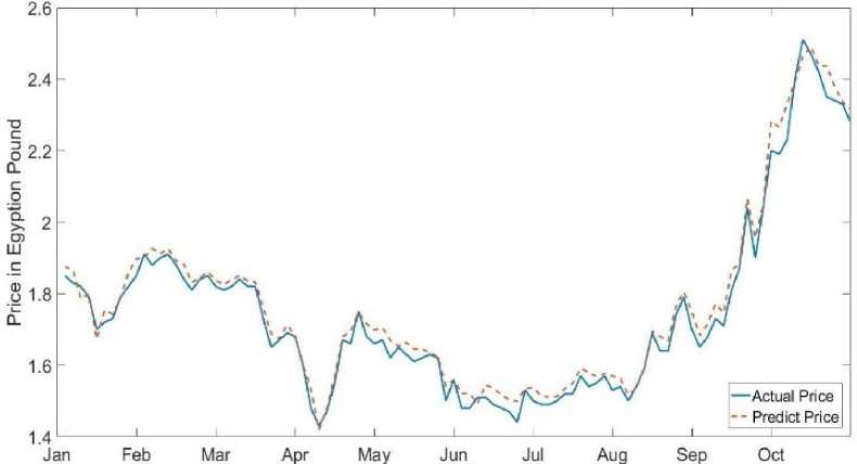
Fig.2. The Predicted and Real Price of APSW by Using Proposed System

Table 1. MSE of Predicted Value of APSW by Using Proposed System

	Number of Epoch	2 Input Network	3 Input Network	4 Input Network	5 Input Network
2 Hidden Units	1000 epoch	0.001882	0.002375	0.136248	0.007366
	5000 epoch	0.001861	0.002623	0.002899	0.002321
	10000 epoch	0.00188	0.0024	0.013596	0.005476
	20000 epoch	0.001935	0.002651	0.002661	0.002108
3 Hidden Units	1000 epoch	0.001879	0.002209	0.002537	0.007513
	5000 epoch	0.002153	0.001779	0.013517	0.01433
	10000 epoch	0.001911	0.002061	0.006972	0.039386
	20000 epoch	0.001854	0.002272	0.00246	0.019161
4 Hidden Units	1000 epoch	0.002366	0.002752	0.005151	0.004487
	5000 epoch	0.001987	0.003541	0.002075	0.011632
	10000 epoch	0.002128	0.001735	0.002548	0.008316
	20000 epoch	0.00215	0.005418	0.182045	0.002523
5 Hidden Units	1000 epoch	0.002345	0.002227	0.359413	0.003696
	5000 epoch	0.003066	0.005668	0.00276	0.016487
	10000 epoch	0.002495	0.002698	0.092086	0.020651
	20000 epoch	0.002528	0.00317	0.002366	0.001883
6 Hidden Units	1000 epoch	0.00209	0.001724	0.00266	0.002785
	5000 epoch	0.002092	0.00327	0.010587	0.004059
	10000 epoch	0.003952	0.001908	0.003677	0.0092
	20000 epoch	0.004079	0.008066	0.001879	0.003479
7 Hidden Units	1000 epoch	0.005634	0.002191	0.001838	0.036597
	5000 epoch	0.002162	0.002363	0.008796	0.12004
	10000 epoch	0.002852	0.050816	0.002419	0.004452
	20000 epoch	0.004569	0.002829	0.003665	0.199039
8 Hidden Units	1000 epoch	0.005034	0.00219	0.01628	0.008163
	5000 epoch	0.003846	0.020369	10.66238	0.003617
	10000 epoch	0.003093	0.003336	0.047447	9.359952
	20000 epoch	0.001986	0.001737	0.033	0.065703
9 Hidden Units	1000 epoch	0.009158	0.011002	99.29887	0.050166
	5000 epoch	0.003107	0.031303	0.009273	0.00524
	10000 epoch	0.260278	0.003504	1.610167	0.364813
	20000 epoch	0.003906	0.002762	0.953	0.883598
10 Hidden Units	1000 epoch	0.002958	0.016061	0.024339	0.190392
	5000 epoch	0.002146	0.020701	0.311	0.2001
	10000 epoch	0.003384	0.102616	0.0464	0.003196
	20000 epoch	0.003378	0.002606	0.788075	0.068603

Table 2. MSE of Predicted Value of AFDI by Using Proposed System

	Number of Epoch	2 Input Network	3 Input Network	4 Input Network	5 Input Network
2 Hidden Units	1000 epoch	0.021947	0.019404	0.028204	0.027051
	5000 epoch	0.020336	0.021537	0.041995	0.024271
	10000 epoch	0.024133	0.020696	0.028393	0.020078
	20000 epoch	0.021651	0.177448	0.02281	0.019571
3 Hidden Units	1000 epoch	0.021714	0.109878	0.0237	0.036911
	5000 epoch	0.022819	0.84517	0.10413	0.020288
	10000 epoch	0.024156	0.022253	0.025612	0.022312
	20000 epoch	0.024428	0.020607	0.018711	0.033687
4 Hidden Units	1000 epoch	0.031942	0.020242	0.018601	0.033454
	5000 epoch	0.021581	0.019363	0.022332	0.026332
	10000 epoch	0.022756	0.024268	0.023732	0.180472
	20000 epoch	0.028871	0.023095	0.031151	0.017572
5 Hidden Units	1000 epoch	0.028584	0.044131	0.026302	0.032294
	5000 epoch	0.030403	0.022422	0.019004	0.250389
	10000 epoch	0.022891	0.025216	0.02931	0.031126
	20000 epoch	0.030691	0.029175	0.170235	0.069502
6 Hidden Units	1000 epoch	0.026276	0.019538	0.06047	0.02948
	5000 epoch	0.021687	0.018398	0.031878	0.044291
	10000 epoch	0.021819	0.026271	0.022179	0.15899
	20000 epoch	0.024998	0.043651	0.055673	0.133115
7 Hidden Units	1000 epoch	0.02627	0.119427	0.028744	0.092296
	5000 epoch	0.025249	3012.623	0.083991	0.035706
	10000 epoch	0.025551	0.022322	0.025876	1.536513
	20000 epoch	0.021602	0.021704	0.033393	10428.53
8 Hidden Units	1000 epoch	0.024245	0.024205	0.060769	0.08655
	5000 epoch	0.027045	0.029882	0.040683	0.09766
	10000 epoch	0.046768	0.95972	0.027265	0.6925
	20000 epoch	0.056252	0.028679	0.031184	0.030349
9 Hidden Units	1000 epoch	0.439601	0.075547	0.045314	0.484801
	5000 epoch	0.074946	0.020189	0.063909	0.118255
	10000 epoch	0.0604	0.022808	0.027645	0.107475
	20000 epoch	0.030325	0.190639	0.02156	0.102232
10 Hidden Units	1000 epoch	0.025853	0.095796	0.032715	0.687401
	5000 epoch	0.029063	0.597869	0.082724	0.04836
	10000 epoch	0.02373	0.027377	0.292866	0.487553
	20000 epoch	0.043628	0.656717	0.039819	0.377600

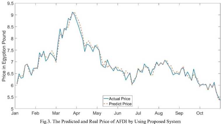
Table 3. Comparison in MSE between Traditional neural network and Heretical structure of neural network

	Traditional neural network	Heretical structure of neural network
Arabia Lahalig Alactan (ACGC)	0.014335	0.004493
Arabia Wa Polivara Lalghazle Wa Elnasig (APSW)	0.0083	0.0017
Alahely Laltanmia Wa Alstasmar (AFDI)	0.101413	0.0184

Table 4. Comparison in training time between Traditional neural network and Heretical structure of neural network in serial and parallel mode

Traditional neural network Heretical structure of neural network in serial mode Heretical structure of neural network in parallel mode Arabia Lahalig Alactan (ACGC) 34.8950 sec 41.6383 sec 32.8905 sec Arabia Wa Polivara Lalghazle Wa Elnasig (APSW) 181.6082 sec 63.6710 sec 30.2684 sec Alahely Laltanmia Wa Alstasmar (AFDI) 178.5513 sec 64.0604 sec 25.7470 sec have to test with even more shares to make sure that our

V.    Conclusion

The prediction quality is efficient for all test shares not only in the prediction values, but also in training time of the network. The neural network is trained within seven year on data points, and tested within three year for all the share and the enhancement in MSE was 68.5% in share of Arabia Lahalig Alactan (ACGC), 79.5% in share of Arabia Wa Polivara Lalghazle Wa Elnasig (APSW) and 81% in share of Alahely Laltanmia Wa Alstasmar (AFDI). Also, the enhancement in training time as 5.7% in share of Arabia Lahalig Alactan (ACGC), 83.3% in share of Arabia Wa Polivara Lalghazle Wa Elnasig (APSW) and 85.6% in share of Alahely Laltanmia Wa Alstasmar (AFDI). Finally, heretical structure of neural network is proven to be very powerful when used for prediction problems of shares daily prices. It improves the Mean Square Error between the real value of price and the predicted value from the system, also it reduces the training time of network when it trains in parallel and also it reduces the complicated structure of neural network because each network learns less data input.

finally in future we need to test the existing methods with more data as the keep coming. We want to ensure that the results we got it is not just a random event. We model can generalize.

Another thing we can do is check how our model works with stocks outside the EGX 30 index. We can try train and evaluate out model with stocks that belong to smaller companies that do not have as many transactions as the big ones. In that case we will be able to see if we can expand our work to other stocks and may be even other stock markets as well