Variational Iteration Method for Solving Differential Equations with Piecewise Constant Arguments

Recently, there has been much research concerning properties of solutions of differential equations with piecewise constant arguments (EPCA) [1-4]. In these equations, the derivatives of the unknown functions depend on not just the time t before t . Since this is essentially expressing the derivatives on terms of the solution at discrete points of time before t , it is usually referred to as a hybrid system, other examples of the application of these equations to the problems of biology, cellular neural networks and mechanical systems can be found in [5-8] .

EPCA has been under intensive investigation for the last twenty years. The first studies in this field have been given in [9,10], after this, stability, contractivity and existence of periodic solutions have been treated by several authors, see [11-13] and references therein. The general theory and basic results for EPCA have been thoroughly investigated in the book of Wiener[14]. Nowadays, much research has been focused on the

* Corresponding author.

numerical solutions of EPCA, including convergence[15], stability[16] and oscillation[17]. However, we can’t find any results concerning the approximate anaytical solution of EPCA have been published. In our paper, we will apply the well-known anaytical approximate technique: the variational iteration method to the follwing EPCA:

u ’(t) = au(t) + bu([“]), t - 0, u (0) = u0, where a, b, u^ G R and [•] denotes the greatest integer function.  The main goal of this paper is to extend the variational iteration method to find the solution of (1).

The variational iteration method (VIM) [18-21], which is a well-established technique with wide applications for ordinary differential equations, partial differential equations and delay differential equations, etc. More materials of the classical solution techniques that are most commonly used to solve equations and systems, such as the Adomian decomposition method (ADM) are found in [22], Differential transformation method (DTM) [23], Homotopy analysis method (HAM) [24] and the Homotopy perturbation method (HPM) [25]. The VIM is the most e ff ective and convenient one for both weakly and strongly nonlinear equations. This method has been shown to e ff ectively, easily, and accurately solve a large class of linear and nonlinear problems.

• 2.    PrelimInaries

Definition 1 [14] A solution of (1) on [0, ^ ) is a function u ( t ) that satisfies the conditions:

• (i)    u ( t ) is continuous on [0, ^ ) ,

• (ii)    The derivative u '( t ) exists at each point t G [0, to ) , with the possible exception of the point t = 2 n , n = 0,1, • * • , where one-sided derivatives exist,

• (iii)    Eq. (1) is satisfied on each interval [2 n , 2( n + 1)) c [0, to ) .

• 3.    VARIATIONAL ITERATION MRTHOD (VIM)

Theorem 1 [14]. If a <  0,| b | < — a , then the solution of (1) tends to zero as t ^ to for any given u₀

The VIM is the general Lagrange method, in which an extremely accurate approximation at some special point can be obtained, but not an analytical solution. To illustrate the basic idea of the VIM we consider the following general differential equation

Lu + Nu = g ( x )                                                               (2)

where L and N are linear and nonlinear operator, respectively, and g ( x ) is the inhomogeneous term. In [26–29], the author proposed the VIM where a correction functional for (2) can be written as

x

• u_n + 1 ⁽ x ) = u n ⁽ x ) + I ^X(t ^)[ Lu n ^(t ) + Nu n ^{( t} ) ^— g^(t)]dt                                            (3)

where X is a general Lagrange’s multiplier, which can be identified optimally via the variational theory, and u n as a restricted variation which means ^u n = 0 . It is to be noted that the Lagrange multiplier X can be a constant or a function.

The VIM should be employed by following two main steps. It is required first to determine the Lagrange multiplier X that can be identified optimally via integration by parts and by using a restricted variation. Having X determined, an iteration formula, without restricted variation, should be used for the determination of the successive approximations u(x) of the solution u(x). The zeroth approximation u can be any selective function. Consequently, the solution is given by u (x) = lim un (x) .

n ^да

Now, we apply the VIM to (1) . A correction functional is constructed as follows: ts u +i(t) = un (t) +  X(s)[u (s) - aun (s) - bun ([—])]ds.

n ^{+ 1}           n        00                                         2

Taking variational on both sides of (5), we have t'

5u,(t) = Sun (t) + 5  X(s)u (s)ds, nn0n

= 5u (t) + X(t)5u (t) - Г X'(s)5u„ (s)ds, n                 n0           n

= (1 + X(t))5u (t) - ft X'(s>„ (s)ds, n0           n this yields the stationary conditions:

''1 + X ( t ) = 0,

X s ) , = t = 0.

Thus

X( s) = -1, and we obtain the following iteration formula t'

u„+1 (t) = un (t) -  [u (s) - aun (s) - bun ([-])]ds.

0n2

So we have u 0( t ) = u 0, t'

u (t) = uo(t) -  [u (s) - au0 (s) - bu0 ([-])]ds, t'

u ₂ ( t ) = u_x ( t ) -   [ u ( s ) - au_x ( s ) - bu_x ([—])] ds ,

• 2           1          01              11

t'

u ₃ ( t ) = u ₂ ( t ) -   [ u ( s ) - au ₂ ( s ) - bu ₂ ([—])] ds ,

• 3         2        02            22

u ( t ) = lim u_n ( t ) .

n ^ro

In order to overcome the difficulty from the greatest integer function [ • ] , we can consider the above iteration formula in a series of intervals : [0,2) , [2,4) , [4,6) , _, [2 n , 2( n + 1)) where n = 0,1,2, ^. Following this way, each integral in iteration formulas will be easily computed.

The above analysis yields the following theorem:

Theorem 2 . The VIM solution of (1) can be determined by (9) with the iterations (8).

In the next section, the VIM is successfully applied for solving a linear EPCA.

4. APPLICATION

In what follows, we will apply the VIM method to a physical model to illustrate the strength of the method.

Let a = 2 , b = - 3 and U _o = 1 in (1), this in turn gives the successive approximations by (8).

When 1 e[0,2), u1,0( t) = 1, u1,1(1) = u1,0 (1) - C[u' 0 (5) - 2u1,0 (s) + 3u1,0 ([s])]ds ,                     ,                  0      1,0                       ,,

= ^1- J ₀ ^{(-2+3) ds}

= 1 -1, u1,2(t) = u (t) - Г[u (s) - 2и1Д (s) + 3ихл ([s])]ds

,                         ,                     0        1,1                           ,,

= 1 - 1 -

J_o t [- 1 — 2(1 - s ) + 3^ , (0) ] ds

= 1 - 1 - 1 ²,

U 13 ( t ) = U 12 ( t ) - f [ и  ( s ) - 2 U 12 ( s ) + 3u_V 2 ([ s ])] ds

,                     ,                  0      1,2                       ,,

= U j 2 ( t ) - J |^- 1 - 2 s - 2(1 - s - s ²) + 3 и 2(0) ^ ds = 1 - 1 - 1 ² - ~ t ³,

^U 1,4 ^{( 1} ) = ^U 1,3 ^{( 1} ) ^- f ^{1 [ U} ' ₃^{( s} ) ^{- 2 u} 1,3 ^{( s} ) ^{+ 3 u} 1,3 ^([ s ^{])] ds}

,                   ,                0     1,3                    ,                     ,

U\,3

⁽ t ) - l o t - 3

t

= 1 — t — t ²-- t³

4 2          ^xx   ,

+ j s + 3 ц ₃(0) ds

3   ,

When 1 e [2,4) ,

^U 2,o^{( 1} ) = 1,

s

⁽ 5 ) ^- 2 ^u2 0 (s) + 3 u 2,o ([-D] d ^s

^U 2,1^{( 1} ) = ^U 2,0 ^{( 1} ) ^- J₀ t ^{[ U}

= ¹ - Jo ^{(-2 + 3)} ds

= 1 - t ,

^U 2,2 ^{( 1} ) = ^U 2,1 ^{( 1} ) - f t ^{[ U}' , ⁽ s ) - ^{2 U} 2,1 ⁽ s ) ^{+ 3u} 2,1 ^{([ 5 ])]} ds ,                   ,               0       2,1                      ,                     ,

= 1 -t - J [-1 — 2(1 — s) + 3u21 (1)] ds

= 1 + 2 t - 1 ²,

ts u2,3 (1) = u2,2 (1) -J [u2,2 (s) — 2u2,2 (s) + 3u2,2 ([^ds

= u^ ₂ ( 1 ) - J ¹ [ 2 - 2 s - 2(1 + 2 s - s ²) + 3 u _{2 2} (1) ] ds

= 1 - 4 1 + 2 1 ² - 2 1 ³,

t'                                            s u2,4 (1) = u2,3 (1) -J [\3 (s) - 2u2,3 (s) + 3u2,3 ([^ds

= u 2,3 ^{( 1} ) - L

- 6 + 12 s - 6 s + — s + 3 u ₂₃(1) ds

= 1 + 7 1 - 4 1 ² + ⁴ 1 ³ -¹ 1 ⁴, 33

When 1 e[4,6), u 30( 1) = 1

u 3,1 ⁽ t ) = u 3,0 ⁽ t ) ^- J_o ^{1 [} u 3,₀^{( s} ) ^{- 2} u 3,0 ^{( s} ) ^{+ 3} u 3,0 ^([ s ^{])] ds}

= ¹ - J ( - 2 + ³ ) ds = 1 - 1 ,

t'                                          s u3,2 (1) = u3,1 (1) - In [u3 , (s) - 2u3,1 (s) + 3u3,1 ([-])]ds

^{,                   ,}                ₀       3,1                      ^{,                     ,}       ₂

= u 3,1 ( 1 ) - Jo [- 1 - 2(1 - s ) + 3 u 3,1 (2) ] ds = 1 + 5 1 - 1 ²,

u 3,3 ( 1 ) = u 3,2 ( 1 ) - f_n [ u ' ₂ ( s ) - 2 u 3,2 ( s ) + 3 u 3,2 ([ s ])] ds ,                      ,                  0       3,2                         ,                         ,

= u3,2(1)-Jd[5-2s-2(1 + 5s-s2) + 3u32(2)]ds = 1 -191 + 512 -113, u3,4 (1) = u3,3 (1) - J1 [u' 3 (s) - 2u3,3 (s) + 3u3,3 ([s])]ds

^{,                   ,}                 ₀      3,3                      ^{,                      ,}        ₂

=u3,3( о - L

—21 + 48 s —12 s + — s + 3 u^ ₃(2) ds

= 1 + 69 1 - 19 1 ² + 1° 1 ³ - 1 1 ⁴, 33

In a word, in the interval [2 n , 2( n + 1)) , n = 0,1,2, we have the following iteration formulas:

un +1,0( t) = 1, un +1,m (t) = un +1,m-1 (t)

-Jo [ u n + 1m - 1 ⁽ s ) - 2 u n + 1, m - 1 ⁽ s ) ^{+ 3} u n + 1, m - 1 ⁽ n ^{)] ds}

In view of (9), we can obtain the approximate analytical solution. Usually, the m + 1 th approximation is used for numerical purposes.

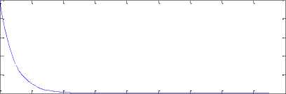
In Table 1, we compare the absolute errors of the VIM ( m = 4,5) with the ones of the 1-Gauss-Legendre method[16] using h = 0.02 . The graphs of the exact solution and 7th approximate solutions are shown in Fig. 1.

Table. 1.Comparison of the absolute errors

t	VIM		1-Gauss- Legendre method
	m=4	m=5
0.7	3.09E-6	5.47E-7	2.33E-4
1.4	4.14E-6	7.72E-7	4.16E-4
2.1	5.16E-6	5.17E-6	3.81E-3
2.8	4.34E-5	6.14E-6	5.42E-3
3.5	5.51E-5	8.75E-6	8.15E-3
4.2	7.36E-5	1.08E-5	1.96E-2
4.9	3.84E-4	2.92E-5	2.37E-2
5.6	8.26E-4	6.52E-5	4.73E-2

0.8

0.6

0.4

0.2

0.8

0.6

0.4

0.2

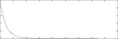
Fig. 1. Comparison of the exact solution with the VIM solution, Upper: exact solution, Lower: 7th VIM solution

• 5.    CONCLUSION

In this paper, we have demonstrated the feasibility of the VIM for solving a EPCA model. We obtain high-accuracy approximate solutions. The numerical results also show that the VIM offers a very effective and convenient approach to the approximate solution of EPCA.