Varna-based optimization: a new method for solving global optimization

Author: Ashutosh Kumar Singh, Saurabh, Shashank Srivastava
Journal: International Journal of Intelligent Systems and Applications @ijisa
Article in issue: 12 vol.10, 2018.
Free access
A new and simple optimization algorithm known as Varna-based Optimization (VBO) is introduced in this paper for solving optimization problems. It is inspired by the human-society structure and human behavior. Varna (a Sanskrit word, which means Class) is decided by people’s Karma (a Sanskrit word, which means Action), not by their birth. The performance of the proposed method is examined by experimenting it on six unconstrained, and five constrained benchmark functions having different characteristics. Its results are compared with other well-known optimization methods (PSO, TLBO, and Jaya) for multi-dimensional numeric problems. Our experimental results show that the VBO outperforms other optimization algorithms and have proved the better effectiveness of the proposed algorithm.
VBO, optimization, constrained benchmark, unconstrained benchmark
Short address: https://sciup.org/15016548
IDR: 15016548 | DOI: 10.5815/ijisa.2018.12.01
Text of the scientific article Varna-based optimization: a new method for solving global optimization
Published Online December 2018 in MECS
The term “optimization” means finding optimal solutions from all feasible solutions based on their objective(s). Any optimization problem has a set of a specific number of goals (one or more objective functions), a search domain (one or more feasible solutions) and a search method (optimization algorithms). Most of the traditional optimization techniques fail to solve large problems. Therefore, still, there is the requirement of efficient and effective optimization methods to solve such large problems. There are numerous heuristics based optimization algorithms, and these algorithms can be classified based on their principles such as population-based, iterative based, stochastic-based, etc. An algorithm gives the set of solutions (population) and tries to improve these solutions is known as population-based technique. An algorithm which uses multiple iterations to provide better solutions is called an iterative-based method, and by using randomness, the algorithm gives better solutions is known as a stochastic-based method. There is another classification of heuristic approach which is based on nature, and it is called nature-inspired. Population-based nature-inspired algorithms are categorized into two main groups: 1) Evolutionary Algorithms (EA) and 2) Swarm Intelligence (SI) based algorithms. Some of the popular Evolutionary algorithms are Genetic Algorithm (GA)[1], Differential Evolution (DE)[2], Artificial Immune Algorithm (AIA)[3], Evaluation Strategy (ES)[4], Bacteria Foraging Optimization (BFO)[5], Evolution Programming (EP)[6], Grenade Explosion Method (GEM)[7], and so on. Some of the popular Swarm Intelligence (SI) based algorithms are Particle Swarm Optimization (PSO)[8], Artificial Bee Colony (ABC)[9], Shuffled Frog Leaping (SFL)[10], Firefly Algorithm (FA)[11], Ant Colony Optimization (ACO)[12], and so on. All these algorithms use their own controlling parameters.
GA is most popular optimization technique which comes under EA. Working of GA is based on Darwin’s principle of survival of the fittest [6]. GA uses controlling operators such as mutation, crossover, and selection. DE is a population based algorithm which is most widely used to solve the constrained optimization problems whose objective functions such as non-continuous, nonlinear, and non-differentiable, have many local optima, etc. Theory of AIA is inspired from the immune system of the human being. Working of ES is based on the concepts of evolution and adaptation. BFO is motivated by the social foraging behavior of bacteria. EP is also a global optimization method, and it is similar to GA. GEM is inspired by the observation of a grenade explosion.
Dr. Eberhart and Dr. Kennedy developed PSO in 1995, and PSO is also a population-based optimization method. The idea of PSO is motivated by the social behavior of bird flocking. It uses the concept of personal and social experience. ABC is motivated by the foraging behavior of a honey bee. In ABC, the colony is classified into three groups such as employed bees, onlookers, and scouts. The idea of SFL is based on watching, copying, and forming the behavior of a group of frogs that are searching for the location that has the maximum amount of available food. The theory of FA is based on the flashing behavior of fireflies. ACO is inspired by the foraging behavior of the ants that are searching for the food.
Authors of [13] used the GA to solve the medical field problem. Also, their objective is to search the features (or genes) that can predict the type of patient. Rao et al. [14] introduced a Teaching-learning-based optimization (TLBO) in 2011. It is a population-based algorithm that is inspired by the behavior of a teacher and learners. It uses a population of solutions to proceed to the global optima. But, in one iteration, TLBO does twice number of function evaluations than PSO. Rao [15] introduced Jaya algorithm in 2015 which is also a population based optimization method where the philosophy is to move towards the best solution and away from the worst solution.
Previously, most of the heuristic approaches consider the same formulation for all the particles in the population. To work a system well, all components of the system need not do the same task, a variation in their task may improve the performance. We utilized this concept in our proposed algorithm. We get inspired by the working of human society and their behavior, where people are assigned specific tasks for development of the society. In this paper, Varna-based Optimization (VBO) algorithm is proposed to find the optimal global solution for the constrained and unconstrained optimization problems. VBO algorithm is based on human societystructure and behavior. VBO algorithm and its working are explained in detail in next section.
The main contributions of this paper are summarized as:
-
• We develop a new and simple optimization algorithm named Varna-based Optimization (VBO) and use it for solving the optimization problems.
-
• We compare PSO, TLBO, and Jaya algorithms with our proposed algorithm (VBO) where the performance of VBO is found to be better.
The rest of the paper is structured as follows. In this paper, we present the overview of VBO in section II. In section III, we demonstrate the working of VBO. Section IV shows the experimental results and discussions. Finally, the paper is concluded in section V.
-
II. Varna Based Optimization
In proposed algorithm, particles in the population are classified into two Varna (a Sanskrit word, which means Class), namely class A and class B. This classification is based on the superiority of particles. Particles having better fitness value belongs to class A (like elite group), and rest particles belong to class B. The particles in a particular class follow rules of that class and work accordingly. Also, it is not necessary that particles present in a particular class in present generation will always remain in it. In the next generation, it may go to other class as well. So, Varna is decided by particle’s Karma (Fitness value), not by their birth.
For example, we consider the human society of 12 people (two of them belong to the elite group and remaining ten people belong to a normal group) as shown in Fig.1. So, class A has two people, and class B has ten people. According to human social structure and its behavior, it is not necessary that people always present in their particular group. People’s Varna is decided by their Karma , not by their birth. If an individual from normal group performs well, then it is promoted to elite group and the low performer individual from elite group goes to normal group as shown in Fig. 2 and Fig. 3. This transitioning keeps on happening based on the performance of the individuals.
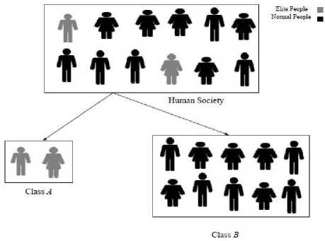
Fig.1. Initial classification of human society such as class A and class B
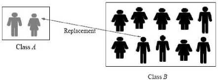
Fig.2. Replacement of human from class A to class B based on their Karma (Action)
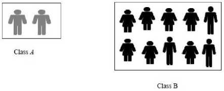
Fig.3. Classification of class A and class B after some generations
Here, the task for class A is exploitation and for class B is exploration. The particles in class A have the property to move towards the best solution and away from the worst solution. On the other hand, particles in class B interact whole population peer to peer, and their movement is decided by fitness value of respective peer particles. For deciding the sizes of classes, we take a fixed fraction (α) of the population in class A and rest in class B. We recommend the value of α to be from 0.05 to 0.20, in this paper we set α = 0.10 for the experiment. And we set peer constants as c1 = 1.50 and c2 = 1.25. The values for c1 and c2 are kept higher than one to cover the search regions around the better counterpart. The value of c1 is still kept higher than c2 as there is more chance of promising solution around particle having the best solution.
Particles in class A move towards the best solution and simultaneously move away from the worst solution. The random value r ∈ [0,1] is considered for class A . The new positions ( X ′ ) of particles is given by (1).
X ′ = X + r *( X - X ) (1) i i A best worst
For each particles X in class B, we randomly choose a particle from the whole population as X . The random value r ∈ [0,1] is considered for class B. If fitness of X is better than that of X we move that i peer particle towards best solution and away from the peer solution, as in (2).
Xi′=Xi+c1*rB*(Xbest-Xpeer)(2)
If fitness value of X is worse than that of X , we ipeer move that particle towards X peer , as in (3).
Xi′=Xi +c2* rB*(Xpeer -Xi)(3)
If both particles have same fitness value, then new position is updated as in range zero to twice of current position as given in (4).
Xi′=2*rB*Xi(4)
-
III. Demonstration of Working of VBO
In this section, we give the step-by-step procedure of the working of VBO. We use Michalewicz function [16] as given in (5) for the demonstration of our proposed method. Michalewicz function is multi-modal as well as separable but not regular. Fig. 4(a) shows the three dimensional Michalewicz function, and its contour plot with local minima and global minima are shown in Fig. 4(b).
D ix 2
f ( xi ) = - ∑ sin( xi )(sin( i ))2 m i =1 π
The Michalewicz function has D! local minima, where D is the size of the dimension. For larger value of the constant m, the search is more difficult. Here, the value of m is taken as 10.
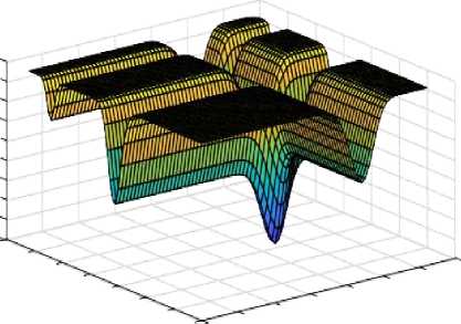
(a) Michalewicz function
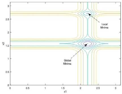
(b) Contour plot
Fig.4. Three Dimensional Michalewicz function and its contour plot
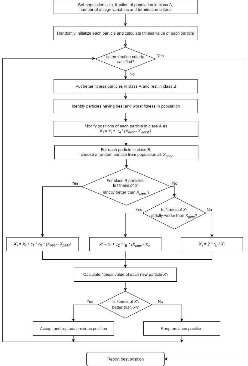
Fig.5. Flow chart of VBO algorithm
Demonstration of working of VBO is as follows:
Step 1: We define the optimization problem and initialize the parameters which are used in this optimization problem. Following parameters are taken for this particular benchmark function i.e. Michalewicz function.
-
• Population size (N) = 12
-
• Number of generations (G) = 20
-
• Number of design variables (d) = 2
-
• Range of design variables ([Lower range, Upper range]) = [0, π ]
-
• Fraction of population of class A ( α ) = 0.10
-
• Random value
-
- rA e [0,1] for class A
-
- rB e [0,1] for class B
-
• Peer constants for class B : cx = 1.50 and c2 = 1.25
Step 2: Randomly initialize each particle (X) and calculate fitness value ( f ( X )) for each of them.
|
x11 |
x 12 |
x 13 |
' x 1 D 1 |
" 0.1818 1.7978 2.5881 0.9428 2.9880 |
1.3721" 1.7752 0.3962 0.0067 2.4074 |
|
x = x 2 1 |
x 22 |
x 23 |
• x 2 D = |
2.3603 |
0.4363 |
|
1.0974 |
0.4755 |
||||
|
_ XN 1 |
xN 2 |
xN 3 |
• xND J |
1.5605 |
2.5405 |
|
1.9882 |
2.1627 |
||||
|
2.0093 |
2.2912 |
||||
|
2.7013 |
1.9696 |
||||
|
_ 0.5673 |
1.8011 J |
|
"-0.2372" |
||
|
- 0.1822 |
||
|
- 0.0188 |
||
|
- 0.0000 |
||
|
and |
- 0.0000 |
|
|
- 0.4660 |
||
|
f ( X )= |
||
|
- 0.0000 |
||
|
- 0.0124 |
||
|
- 0.3387 |
||
|
- 0.3957 |
||
|
- 0.0009 |
||
|
_- 0.0760 _ |
Step 3 : Classify particles into class A and class B . Particles having better fitness value goes into class A and others go into class B . So, sort particles according to their fitness value from best to worst. Select top " 0.10* N "| (here, |" 0.10*12" | = 2) particles for class A and rest for class B .
|
"1.9882 0.1818 1.7978 0.5673 2.5881 |
2.1627" 1.3721 1.7752 1.8011 0.3962 |
and . |
"-0.3387 -0.2372 -0.1822 -0.0760 -0.0188 |
|
|
X = |
f ( X b ) = |
|||
|
B |
1.5605 |
2.5405 |
-0.0124 |
|
|
2.7013 |
1.9696 |
-0.0009 |
||
|
2.9880 |
2.4074 |
-0.0000 |
||
|
1.0974 |
0.4755 |
-0.0000 |
||
|
0.9428 |
0.0067 _ |
_-0.0000 |
Step 4: Identify best and worst solutions:
Xbes t = [2.0093 2.2912]
X wors. = [0.9428 0.0067]
Modify positions of particles in class A , as in (1).
'
Xi = Xi + rA ( Xbest - Xworst ) ^ XA =
2.5921 0.8255
2.1189 2.4367
Step 5: Modify positions of particles in class B as explained in section 2. Let us consider, a particle in class B , Xi = [0.1818 1.3721] with fitness value equal to -0.3387. Let its peer be randomly chosen from the whole population (it can from either class A or class B ) , other than it, as Xpeer = [ 1.0974 0.4755 ] with fitness value equal to -0.0000. As X has better fitness than X , so its new position is given by (2). Similarly, for another particle in class X = [2.7013 1.9696] with fitness value equal to -0.0009. Let its peer be Xpeer = [ 1.9882 2.1627 ] with fitness value equal to -0.3957. Here, X has worse fitness than X , so its new position given by (3).
|
"2.3603 2.0093 1.9882 0.1818 1.7978 0.5673 |
0.4363" 2.2912 2.1627 1.3721 1.7752 1.8011 |
and |
”-0.4660 - 0.3957 - 0.3387 - 0.2372 - 0.1822 - 0.0760 |
|
|
X = |
f ( X )= |
|||
|
2.5881 |
0.3962 |
- 0.0188 |
||
|
1.5605 |
2.5405 |
- 0.0124 |
||
|
2.7013 |
1.9696 |
- 0.0009 |
||
|
2.9880 |
2.4074 |
- 0.0000 |
||
|
1.0974 |
0.4755 |
- 0.0000 |
||
|
0.9428 |
0.0067 _ |
_- 0.0000 |
||
|
"2.3603 |
0.4363 |
"-0.4660 |
||
|
X = |
and f ( X A ) = |
|||
|
A |
2.0093 |
2.2912 |
- 0.3957 |
|
3.0881 |
2.1347 |
|
|
- 0.3180 |
0.7000 |
|
|
1.7218 |
0.2615 |
|
|
0.4568 |
1.7034 |
|
|
2.9062 |
0.5268 |
|
|
X ' = |
||
|
B |
1.5690 |
2.0883 |
|
2.5639 |
1.3843 |
|
|
- 0.0369 |
1.2473 |
|
|
2.5022 |
1.0820 |
|
|
_ 1.1801 |
0.4456 _ |
Step 6: Clamp position values of all particles in both classes within the domain of design variables. And calculate fitness value of each particle.
|
" 2.5921 |
0.8255" |
" -0.0172" |
" 2.3603 |
0.4363" |
"-0.4660 |
||||
|
2.1189 |
2.4367 |
- 0.6979 |
2.1189 |
2.4367 |
- 0.6979 |
||||
|
3.0881 |
2.1347 |
- 0.0000 |
1.9882 |
2.1627 |
- 0.3387 |
||||
|
0.0000 |
0.7000 |
- 0.0000 |
0.1818 |
1.3721 |
- 0.2372 |
||||
|
1.7218 |
0.2615 |
- 0.0145 |
1.7978 |
1.7752 |
- 0.1822 |
||||
|
X ' = |
0.4568 |
1.7034 |
and р , х/ х |
- 0.4573 |
0.4568 |
1.7034 |
- 0.4573 |
||
|
2.9062 |
0.5268 |
f ( X) = |
- 0.0000 |
Xs = |
2.5881 |
0.3962 |
and f ( xs ) = |
- 0.0188 |
|
|
1.5690 |
2.0883 |
- 0.0009 |
1.5605 |
2.5405 |
- 0.0124 |
||||
|
2.5639 |
1.3843 |
- 0.3110 |
2.5639 |
1.3843 |
- 0.3110 |
||||
|
0.0000 |
1.2473 |
- 0.0265 |
0.0000 |
1.2473 |
- 0.0265 |
||||
|
2.5022 |
1.0820 |
- 0.0953 |
2.5022 |
1.0820 |
- 0.0953 |
||||
|
1.1801 |
0.4456 _ |
_- 0.0000 _ |
_ 1.1801 |
0.4456 _ |
_- 0.0000 |
Step 7: Select solutions that give better fitness value than previous solutions as Xs .
Step 8: If termination criteria are met then stop and report the particle having the best solution, otherwise repeat all steps from Step 3 .
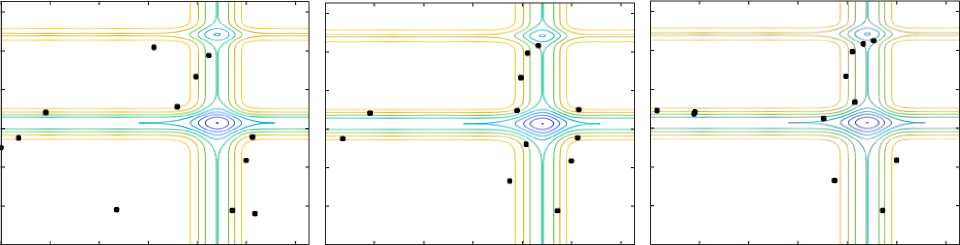
(a) Generation-1 (b) Generation-2 (c) Generation-3
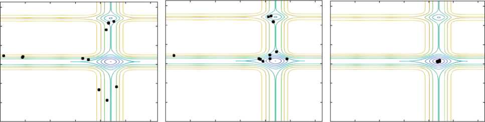
(d) Generation-5 (e) Generation-10 (f) Generation-20
Fig.6. Visualization of convergence of solutions for Michalewicz function for Generation-1, 2, 3, 5, 10 and 20.
Fig. 6 shows the visualization of convergence of solutions for Michalewicz function for generation number 1, 2, 3, 5, 10 and 20. In Generation 1, all 12 particles are randomly distributed over the contour plot of Michalewicz function as shown in Fig. 6(a). In Generation 2, three particles are moving towards local minima, seven particles are moving towards global minima and remaining two particles remain same in their previous position as shown in Fig. 6(b). Similarly, visualization of convergence of particles for Generation 3, 5 and 10 is shown in Figs. 6(c), 6(d), and 6(e) respectively. From these figures, we can see that how rapidly convergence of particles towards global minima is taking place. In Generation 20, all twelve particles have reached to global minima as shown in Fig. 6(f).
Table 1 shows the position and objective function value of particles (as expressed in (5)) for the first two generations (Generation 1 and Generation 2). Here, we consider population size of 12, and it is divided into two classes: class A and class B . First two particles of Generation 1 are in class A and remaining ten particles are in class B . Similarly, the same procedure is followed for generation 2. These two generations give the basic idea of working of proposed VBO algorithm.
Table 1. Variation of design variables and fitness function
|
Generation |
Class |
X |
X |
/(V) |
Xs |
|||||
|
-Г1 |
AZ |
A 4 |
xs xs 1 |
A^) |
||||||
|
A |
f 2.3603 |
0.4363 |
-0.4660 |
2.5921 |
0.8255 |
-0.0172 |
2.3603 |
0.4363 |
-0.4660 |
|
|
[ 2.0093 |
2.2912 |
-0.3957 |
2.1189 |
2.4367 |
-0.6979 |
2.1189 |
2.4367 |
-0.6979 |
||
|
1.9882 |
2.1627 |
-0.3387 |
3.0881 |
2.1347 |
-0.0000 |
1.9882 |
2.1627 |
-0.3387 |
||
|
0.1818 |
1.3721 |
-0.2372 |
0.0000 |
0.7000 |
-0.0000 |
0.1818 |
1.3721 |
-0.2372 |
||
|
Generation 1 |
1.7978 |
1.7752 |
-0.1822 |
1.7218 |
0.2615 |
-0.0145 |
1.7978 |
1.7752 |
-0.1822 |
|
|
0.5673 |
1.8011 |
-0.0760 |
0.4568 |
1.7034 |
-0.4573 |
0.4568 |
1.7034 |
-0.4573 |
||
|
В |
2.5881 |
0.3962 |
-0.0188 |
2.9062 |
0.5268 |
-0.0000 |
2.5881 |
0.3962 |
-0.0188 |
|
|
1.5605 |
2.5405 |
-0.0124 |
1.5690 |
2.0883 |
-0.0009 |
1.5605 |
2.5405 |
-0.0124 |
||
|
2.7013 |
1.9696 |
-0.0009 |
2.5639 |
1.3843 |
-0.3110 |
2.5639 |
1.3843 |
-0.3110 |
||
|
2.9880 |
2.4074 |
-0.0000 |
0.0000 |
1.2473 |
-0.0265 |
0.0000 |
1.2473 |
-0.0265 |
||
|
1.0974 |
0.4755 |
-0.0000 |
2.5022 |
1.0820 |
-0.0953 |
2.5022 |
1.0820 |
-0.0953 |
||
|
[ 0.9428 |
0.0067 |
-0.0000 |
1.1801 |
0.4456 |
-0.0000 |
1.1801 |
0.4456 |
-0.0000 |
||
|
A |
f 2.1189 |
2.4367 |
-0.6979 |
2.1653 |
2.5786 |
-0.8278 |
2.1653 |
2.5786 |
-0.8278 |
|
|
[ 2.3603 |
0.4363 |
-0.4660 |
2.8195 |
2.1284 |
-0.0000 |
2.3603 |
0.4363 |
-0.4660 |
||
|
' 0.4568 |
1.7034 |
-0.4573 |
0.0000 |
1.7123 |
-0.4074 |
0.4568 |
1.7034 |
-0.4573 |
||
|
1.9882 |
2.1627 |
-0.3387 |
2.7097 |
2.0211 |
-0.0006 |
1.9882 |
2.1627 |
-0.3387 |
||
|
2.5639 |
1.3843 |
-0.3110 |
1.9315 |
2.1103 |
-0.2073 |
2.5639 |
1.3843 |
-0.3110 |
||
|
Generation 2 |
0.1818 |
1.3721 |
-0.2372 |
0.6081 |
1.3458 |
-0.1614 |
0.1818 |
1.3721 |
-0.2372 |
|
|
В |
1.7978 |
1.7752 |
-0.1822 |
2.5751 |
1.7488 |
-0.2557 |
2.5751 |
1.7488 |
-0.2557 |
|
|
2.5022 |
1.0820 |
-0.0953 |
2.5321 |
1.2266 |
-0.0745 |
2.5022 |
1.0820 |
-0.0953 |
||
|
0.0000 |
1.2473 |
-0.0265 |
1.9503 |
1.7366 |
-0.5310 |
1.9503 |
1.7366 |
-0.5310 |
||
|
2.5881 |
0.3962 |
-0.0188 |
2.0560 |
2.4814 |
-0.5307 |
2.0560 |
2.4814 |
-0.5307 |
||
|
1.5605 |
2.5405 |
-0.0124 |
1.8747 |
0.8225 |
-0.1148 |
1.8747 |
0.8225 |
-0.1148 |
||
|
[ 1.1801 |
0.4456 |
-0.0000 |
2.0421 |
1.3001 |
-0.5648 |
2.0421 |
1.3001 |
-0.5648 |
||
-
IV. Experimental Results and Discussions
In this section, we have performed different experiments on unconstrained and constrained benchmark functions to check the effectiveness of VBO with other optimization algorithms. These benchmark functions have different characteristics and functionality such as uni-modal, multimodal, separable, non-separable, regular, non-regular and so on. A function is having only one local optima (minima or maxima) is called uni-modal and more than one local optima are called multi-modal. A function is regular, if it differentiable at every point of its search space otherwise non-regular.
-
A. Experimental setup
-
• Used a 64-bit Windows 8.1 operating system running Intel Core i7-4770 CPU @ 3.40 GHz having 16 GB RAM.
-
• Used MATLAB 2017a as a platform for coding the algorithms and plotting graphs.
-
• Maximum number of function evaluations set
o 100000 for unconstrained benchmark functions o 200000 for constrained benchmark functions
-
-
• Population size taken as 100.
-
B. Experiments on unconstrained benchmark functions
We have used six well-known unconstrained benchmark functions with different functionality and characteristics. Details of these functions considered by Akay and Karaboga [17] are given in Table 2. In this experiment, to maintain the consistency, we use a common platform for comparison of VBO with other optimization methods such as PSO, TLBO, and Jaya. The performance of proposed VBO algorithm is tested on these six benchmark functions which are well-known in the literature of optimization and compared its results with PSO, TLBO, and Jaya. The performance of VBO is tested for 100 independent runs with the population size of 100, different dimension size (D = 2, 3, 5, 10, 20 and 30) and number of function evaluations is set to 100000.
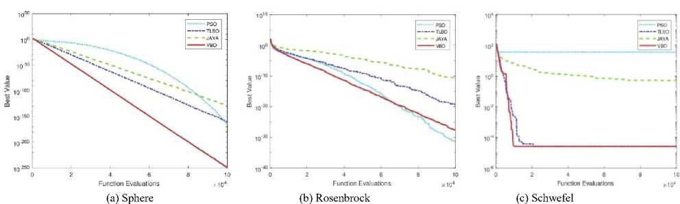
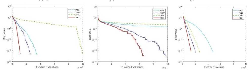
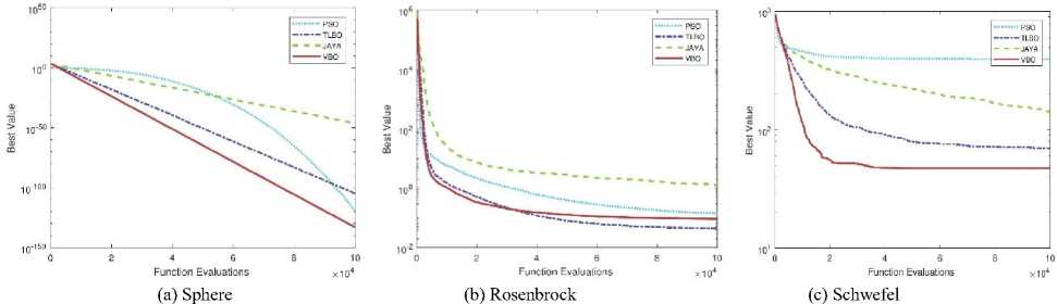
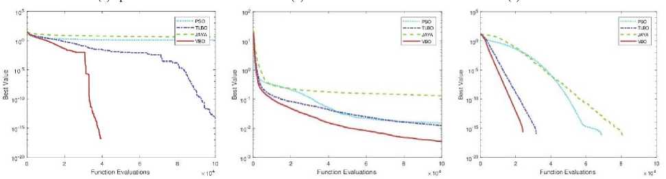
Convergence plots of VBO and other optimization methods (PSO, TLBO, and Jaya) with different dimensions (D = 2, 3, 5, 10, 20 and 30) are shown in Figs. 7, 8, 9, 10, 11 and 12. The performance of VBO and other optimization methods are tested on benchmark functions on the same platform with 100000 function evaluations and averaged over 100 independent runs. We consider the Sphere function and performance of VBO is tested on it with different dimension size (D = 2, 3, 5 and 10). VBO obtained better results as compared to other optimization methods as shown in Figs. 7(a), 8(a), 9(a) and 10(a). When the performance of VBO is tested on Sphere function of dimensions (D = 20 and 30) then initial results of VBO is better than PSO, TLBO and Jaya algorithms. If we increase the size of function evaluations, TLBO is dominated to VBO, but overall, VBO gives better results as compared to PSO and Jaya algorithms as shown in Figs. 11(a) and 12(a).
We consider the Rosenbrock function, and performance of VBO with other optimization methods are tested on the same platform. The performance results of VBO on Rosenbrock function with different dimensions (D = 2, 3, 5, 10, 20 and 30) are shown in Figs. 7(b), 8(b), 9(b), 10(b), 11(b) and 12(b). From these figures, it is observed that VBO gives better results as compared to PSO, TLBO and Jaya algorithms. We use another well-known benchmark function, i.e., Schwefel and test the performance of VBO on it. The performance results of VBO on Schwefel function are shown in Figs. 7(c), 8(c), 9(c), 10(c), 11(c) and 12(c). From these figures, it is clear that VBO is better that PSO, TLBO, and Jaya algorithms.
From Figs. 11(c) and 12(c), it is also observed that VBO gives much better results as compared to PSO, TLBO and Jaya algorithms. Similarly, we test the performance of VBO on Rastrigin function with different dimensions. After experiments, VBO gives better results and dominated other optimization methods (PSO, TLBO, and Jaya) as shown in Figs. 7(d), 8(d), 9(d), 10(d), 11(d) and 12(d). The performance of VBO and other optimization methods is tested on Griewank and Ackley function with different dimensions. The performance results of VBO on Griewank function are shown in Figs. 7(e), 8(e), 9(e), 10(e), 11(e) and 12(e). The performance results of VBO on Ackley function with different dimensions are shown in Figs. 7(f), 8(f), 9(f), 10(f), 11(f) and 12(f). From all these figures as mentioned earlier, it is seen that VBO outperforms other algorithms for all these six unconstrained benchmark functions.
Table 2. Details of benchmark functions considered by Akay and Karaboga [17]
|
Function |
Formulation Search space Multimodal? Separable? Regular? |
|
Sphere |
£ D x 2 [-100, 100] No Yes Yes |
|
Rosenbrock |
£ DD - 1 ( 100 ( x 2 - X i + 1 ) 2 + ( X i - 1 ) 2 ) [-30, 30] No No Yes |
|
Schwefel |
418.9829 D - £ D ( x i sin (J X j) ) [-500, 500] Yes Yes No |
|
Rastrigin |
£ D ( x 2 - 10cos(2 nx ,) + 10 ) [-5.12,5.12] Yes Yes Yes |
|
Griwank |
20 + e - 20exp | O.^^ £ D x 2 j- exp ^ 1 £ D ^os ( 2 n x, ) ^ [-600, 600] Yes No Yes |
|
Ackley |
20 + e - 20exp (- 0.2^-! £ D x 2 ^- exp ^ ^£ D ^os ( 2 n x , ) j [-32, 32] Yes No Yes |

(d) Rastrigin
(f) Ackley
(e) Griewank
Fig.7. Convergence plots of VBO algorithm with other optimization methods on six benchmark functions (D = 2)
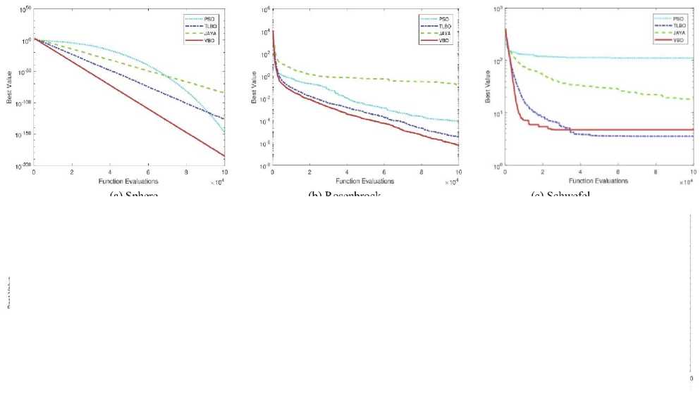
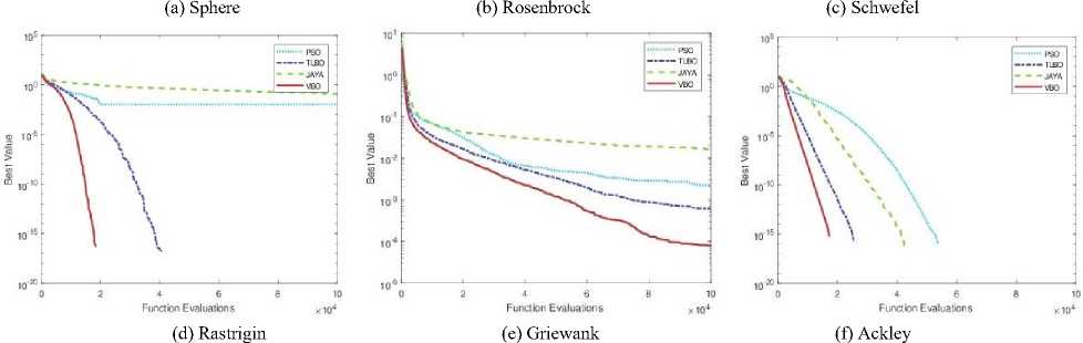
Fig.8. Convergence plots of VBO algorithm with other optimization methods on six benchmark functions (D = 3)
(d) Rastrigin
(f) Ackley
(e) Griewank
Fig.9. Convergence plots of VBO algorithm with other optimization methods on six benchmark functions (D = 5)
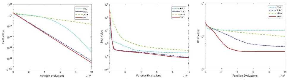
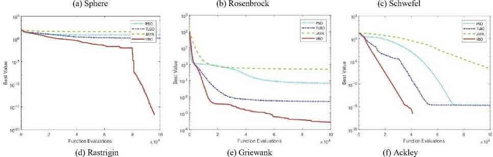
Fig.10. Convergence plots of VBO algorithm with other optimization methods on six benchmark functions (D = 10)
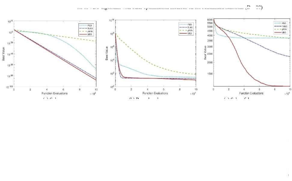
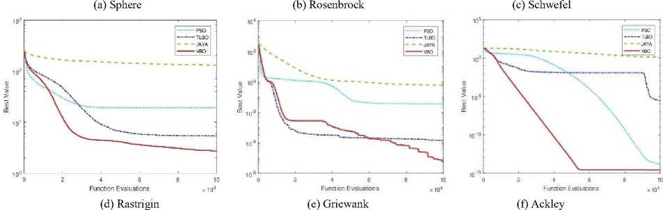
Fig.11. Convergence plots of VBO algorithm with other optimization methods on six benchmark functions (D = 20)
(d) Rastrigin
(e) Griewank
(f) Ackley
Fig.12. Convergence plots of VBO algorithm with other optimization methods on six benchmark functions (D = 30)
Table 3. Comparison of mean and standard deviation of PSO, TLBO, Jaya and VBO for unconstrained six benchmark functions
|
Function |
D |
PSO |
TLBO |
Jaya |
VBO |
||||
|
Mean |
SD |
Mean |
SD |
Mean |
SD |
Mean |
SD |
||
|
2 |
1.69E-166 |
0.00E+00 |
3.71E-161 |
2.23E-160 |
3.16E-129 |
2.65E-128 |
3.13E-250 |
0.00E+00 |
|
|
3 |
1.57E-148 |
8.95E-148 |
2.20E-127 |
1.95E-126 |
2.77E-85 |
1.79E-84 |
2.68E-186 |
0.00E+00 |
|
|
Sphere |
5 |
4.48E-120 |
2.83E-119 |
1.74E-105 |
6.85E-105 |
6.94E-47 |
3.78E-46 |
7.98E-134 |
2.76E-133 |
|
10 |
7.87E-69 |
3.56E-68 |
2.12E-85 |
4.85E-85 |
1.23E-17 |
1.49E-17 |
6.38E-89 |
3.15E-88 |
|
|
20 |
7.74E-26 |
3.89E-25 |
3.38E-70 |
9.14E-70 |
6.86E-04 |
3.36E-04 |
4.04E-56 |
7.88E-56 |
|
|
30 |
1.79E-13 |
1.37E-12 |
2.93E-64 |
3.61E-64 |
2.20E+00 |
8.01E-01 |
5.82E-41 |
9.69E-41 |
|
|
2 |
4.77E-32 |
2.75E-31 |
4.47E-20 |
2.61E-19 |
2.03E-11 |
9.85E-11 |
1.81E-28 |
5.04E-28 |
|
|
3 |
8.49E-05 |
5.89E-04 |
3.41E-06 |
1.03E-05 |
1.50E-01 |
8.82E-01 |
6.13E-07 |
9.56E-07 |
|
|
Rosenbrock |
5 |
1.43E-01 |
2.67E-01 |
4.44E-02 |
3.93E-01 |
1.30E+00 |
3.94E+00 |
9.30E-02 |
5.49E-01 |
|
10 |
3.20E+00 |
9.47E-01 |
6.16E-01 |
8.50E-01 |
7.35E+00 |
9.91E+00 |
5.53E-01 |
8.69E-01 |
|
|
20 |
2.49E+01 |
2.28E+01 |
1.53E+01 |
5.64E-01 |
6.74E+01 |
5.46E+01 |
9.25E+00 |
2.16E+00 |
|
|
30 |
3.63E+01 |
2.40E+01 |
2.60E+01 |
4.04E-01 |
6.60E+02 |
4.32E+02 |
2.47E+01 |
1.61E+01 |
|
|
2 |
3.55E+01 |
5.68E+01 |
2.55E-05 |
0.00E+00 |
4.94E-01 |
2.04E+00 |
2.55E-05 |
0.00E+00 |
|
|
3 |
1.11E+02 |
9.02E+01 |
3.55E+00 |
2.02E+01 |
1.83E+01 |
3.88E+01 |
4.74E+00 |
2.32E+01 |
|
|
Schwefel |
5 |
3.94E+02 |
1.30E+02 |
6.98E+01 |
6.98E+01 |
1.39E+02 |
1.36E+02 |
4.74E+01 |
7.10E+01 |
|
10 |
1.49E+03 |
2.99E+02 |
4.76E+02 |
2.09E+02 |
9.69E+02 |
4.07E+02 |
3.38E+02 |
1.80E+02 |
|
|
20 |
3.73E+03 |
5.14E+02 |
2.31E+03 |
6.74E+02 |
3.66E+03 |
5.73E+02 |
1.08E+03 |
3.24E+02 |
|
|
30 |
5.83E+03 |
8.09E+02 |
4.74E+03 |
1.34E+03 |
7.06E+03 |
6.03E+02 |
2.58E+03 |
9.38E+02 |
|
|
2 |
0.00E+00 |
0.00E+00 |
0.00E+00 |
0.00E+00 |
1.78E-17 |
1.77E-16 |
0.00E+00 |
0.00E+00 |
|
|
3 |
9.95E-03 |
9.90E-02 |
0.00E+00 |
0.00E+00 |
1.22E-01 |
1.56E-01 |
0.00E+00 |
0.00E+00 |
|
|
Rastrigin |
5 |
1.25E+00 |
8.63E-01 |
3.11E-14 |
3.10E-13 |
4.02E+00 |
1.29E+00 |
0.00E+00 |
0.00E+00 |
|
10 |
7.90E+00 |
3.62E+00 |
1.40E+00 |
1.26E+00 |
3.35E+01 |
4.92E+00 |
0.00E+00 |
0.00E+00 |
|
|
20 |
1.92E+01 |
6.47E+00 |
5.34E+00 |
2.67E+00 |
1.31E+02 |
1.14E+01 |
2.69E+00 |
2.85E+00 |
|
|
30 |
3.14E+01 |
1.16E+01 |
7.31E+00 |
4.35E+00 |
2.42E+02 |
1.99E+01 |
7.47E+00 |
3.48E+00 |
|
|
2 |
7.40E-05 |
7.36E-04 |
1.11E-18 |
1.10E-17 |
5.28E-04 |
6.77E-04 |
0.00E+00 |
0.00E+00 |
|
|
3 |
2.19E-03 |
3.55E-03 |
6.10E-04 |
1.91E-03 |
1.62E-02 |
7.04E-03 |
8.03E-05 |
7.37E-04 |
|
|
Griewank |
5 |
1.52E-02 |
8.58E-03 |
1.23E-02 |
7.77E-03 |
1.32E-01 |
3.34E-02 |
3.52E-03 |
4.70E-03 |
|
10 |
6.74E-02 |
2.73E-02 |
5.10E-03 |
8.66E-03 |
4.95E-01 |
8.16E-02 |
2.83E-04 |
2.45E-03 |
|
|
20 |
3.51E-02 |
2.83E-02 |
1.41E-04 |
1.24E-03 |
5.70E-01 |
1.03E-01 |
5.55E-06 |
3.61E-05 |
|
|
30 |
1.37E-02 |
1.40E-02 |
7.51E-05 |
7.47E-04 |
9.78E-01 |
4.94E-02 |
3.26E-04 |
2.94E-03 |
|
|
2 |
-8.88E-16 |
0.00E+00 |
-8.88E-16 |
0.00E+00 |
-8.88E-16 |
0.00E+00 |
-8.88E-16 |
0.00E+00 |
|
|
3 |
-8.88E-16 |
0.00E+00 |
-8.88E-16 |
0.00E+00 |
-8.88E-16 |
0.00E+00 |
-8.88E-16 |
0.00E+00 |
|
|
Ackley |
5 |
-6.04E-16 |
9.64E-16 |
-8.88E-16 |
0.00E+00 |
-6.39E-16 |
9.06E-16 |
-8.88E-16 |
0.00E+00 |
|
10 |
2.66E-15 |
0.00E+00 |
2.24E-15 |
1.15E-15 |
2.37E-07 |
8.86E-07 |
-8.88E-16 |
0.00E+00 |
|
|
20 |
1.44E-14 |
5.18E-14 |
2.86E-06 |
2.80E-05 |
1.22E+00 |
4.11E+00 |
2.59E-15 |
4.97E-16 |
|
|
30 |
2.19E-08 |
8.79E-08 |
3.29E-02 |
2.30E-01 |
3.85E+00 |
4.38E+00 |
2.66E-15 |
0.00E+00 |
|
The comparison of mean and standard deviation (SD) of PSO, TLBO, Jaya and VBO for above mentioned six benchmark functions is given in Table 3. These mean and SD of PSO, TLBO, Jaya, and VBO are obtained from the 100 independent runs of each benchmark functions. From the Table 3, it is clear that overall VBO gives better results as compared to other optimization algorithms (PSO, TLBO, and Jaya) for all six unconstrained benchmark functions.
-
C. Experiments on constrained benchmark functions
We have used five different constrained benchmark functions with different functionality and characteristics. These functions were considered by Liang et al.[18]. In this experiment, we test our proposed VBO algorithm on these five benchmark functions and compare its results with that of PSO, TLBO, and Jaya.
-
1) Constrained benchmark function 1
This test function is minimization problem which is quadratic in nature. It has nine linear inequality constraints and thirteen design variables. The ratio between the feasible region and search space is about 0.0111% [19].
4 413
Minimize f(x)=5∑x -5∑x2 -∑x(6)
i=1 i=1
Subject to g (x)=2x +2x +x +x -10≤ 0
g ( x )=2 x + 2 x + x + x - 10 ≤ 0
g ( x )=2 x + 2 x + x + x - 10 ≤ 0 g 4( x )= - 8 x 1 + x 10 ≤ 0
g 5( x )= - 8 x 2 + x 11 ≤ 0 (7)
g 6( x )= - 8 x 3 + x 12 ≤ 0
g 7( x )= - 2 x 4 - x 5 + x 10 ≤ 0 g 8( x )= - 2 x 6 - x 7 + x 11 ≤ 0 g 9( x ) = - 2 x 8 - x 9 + x 12 ≤ 0
The search space are 0 ≤ xi ≤ 1, where i = 1, 2, 3,... 9, 0 ≤ x i ≤ 100 , where i = 10, 11, 12 and 0 ≤ x 13 ≤ 1. The global minima is at x* = (1 1 1 1 1 1 1 1 1 3 3 3 1) where six constraints are active (g 1 , g 2 , g 3 , g 7 , g 8 and g 9 ) and f( x * ) = - 15.
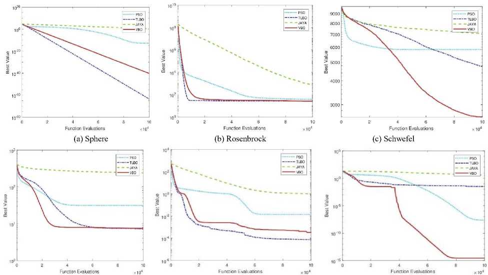
Convergence plots of VBO with other optimization methods (PSO, TLBO, and Jaya) are shown in Fig. 13. VBO, PSO, TLBO, and Jaya algorithms are using the same platform to maintain the consistency. The performance of VBO over other optimization algorithms experiments on function 1, is better as compared to other techniques (PSO, TLBO, and Jaya algorithm) which are shown in Fig. 13(a). From Fig. 13(b), it is observed that VBO gives better results as compared to TLBO and Jaya but not from PSO (for function 2). When we increase the number of function evaluations, then VBO produces almost same results as PSO.
(a) function 1
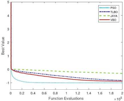
(b) function 2
Fig.13. Convergence plots of VBO algorithm with other optimization algorithms on constrained benchmark function 1 and 2.
-
2) Constrained benchmark function 2
This test function is also a minimization problem which is polynomial in nature. It has one non-linear equality constraint and ten design variables. The ratio between the feasible region and search space is about 0.0000% [19].
n
Minimize ( x ) = - (л/ n ) n ∏ x i i =1
Subject to
h ( x )= ∑ n x 2 - 1=0 (9)
i =1 i
Where, n = 10 and the search space are 0 ≤ x i ≤ 1, where i = 1, 2, 3, ... n. The global minima is at x * = (0.31624357647283069, 0.316243577,...,0.316243576) and f( x * ) = -1.0005001000.
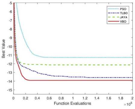
Convergence plots of VBO with other optimization methods (PSO, TLBO, and Jaya) are shown in Fig. 14. VBO, PSO, TLBO, and Jaya algorithms are using the same platform to maintain the consistency. The experimental results on function 3, 4 and 5 show that VBO gives better performance than other optimization algorithms. For function 3 and 4, it is observed that VBO gives better results as compared to Jaya and almost same as PSO and TLBO. For function 5, it is clear that performance of VBO is better as compared to PSO, TLBO and Jaya algorithms.
-
3) Constrained benchmark function 3
This test function is also a minimization problem which is also polynomial in nature. It has four non-linear inequality constraints and seven design variables. The ratio between the feasible region and search space is about 0.5121%.
Minimize f (x) = (x -10)2 + 5(x2 -12)2 + x34
+ 3( x 4 -11)2 + 10 x 5 6 + 7 x 2'
+ x7 - 4 x6x7
-
- 10 x, - 8 x7
Subject to gx (x) = -127 + 2 x 2 + 3 x4 + x3
-
+ 4 x ^ + 5 x 5< 0
g 2 ( x ) = - 282 + 7 xx + 3 x 2 + 10 x 3 2
+ x4 - x 5< 0
g 3 ( x ) = - 195 + 23 xx + x 2 + 5 x 2
-
- 8 x 7< 0
-
g 4 ( x ) = 4 x 2 + x 2 - 3 xxx2 + 2 x 3 2
+ 5 x 6 -11 x 7< 0
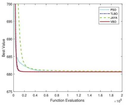
(a) function 3
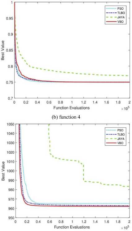
(c) function 5
Fig.14. Convergence plots of VBO algorithm with other optimization algorithms on constrained benchmark function 3, 4 and 5.
The search space is -10 < x i < 10, where i = 1, 2,...,7. The global minima is at x * = (2.3304993 5147405174, 1.95137235847114592,...,1.5942255780571519) and f( x * ) = 680.630057374402. Two constraints (g1 and g4) are active.
-
4) Constrained benchmark function 4
This test function is minimization problem which is quadratic in nature. It has only one non-linear equality constraints and two design variables. The ratio between the feasible region and search space is about 0.0000%.
Minimize f (x) = x2 + (x2 -1)2 (12)
Subject to
h ( x ) = x 2 - x 2 =0 (13)
The search space is -1 < x 1 , x 2 < 1. The global minima is at x* = (-0.7070350700, 0.5000000043) and f( x* ) = 0.7499.
-
5) Constrained benchmark function 5
This test function is minimization problem which is quadratic in nature. It has one linear and one non-linear equality constraint and three design variables. The ratio between the feasible region and search space is about 0.0000%.
Minimize
( x ) = 1000 - x 2 - 2 x 2 - x 2 - xx - xx3 (14)
Subject to h (x) = x12 + x2 + x2 - 25 = 0
h ( x ) = 8 x + 14 x 2 + 7 x 3 - 56 = 0
The search space is 0 ≤ x i ≤ 10; i = 1, 2, 3. The global minima is at x * = (3.51212, 0.21698, 3.55217) and f( x * ) = 961.71502.
As shown in Figs. 14(a) and 14(b), it is observed that VBO gives better results as compared to Jaya algorithm and almost same as PSO and TLBO algorithms. Fig. 14(c), clearly shows that performance of VBO is better than PSO, TLBO and Jaya algorithms. Comparison of mean and SD of PSO, TLBO, Jaya and VBO for these five constrained benchmark functions are given in Table 4.
Table 4. Comparison of mean and standard deviation of PSO, TLBO, Jaya and VBO for constrained five benchmark functions
|
Function |
PSO |
TLBO |
Jaya |
VBO |
|
|
Best |
-15.000002 |
-15.000002 |
-15.000002 |
-15.000002 |
|
|
Worst |
-7.000003 |
-9.453129 |
-5.235363 |
-9.453129 |
|
|
function 1 |
Mean |
-11.277191 |
-13.584221 |
-12.136220 |
-13.913284 |
|
SD |
1.734421 |
1.351544 |
2.345873 |
1.234300 |
|
|
Median |
-10.828129 |
-13.414066 |
-12.031023 |
-15.000002 |
|
|
Best |
-1.000062 |
-1.000030 |
-0.862619 |
-1.000021 |
|
|
Worst |
-1.000043 |
0.000000 |
0.000004 |
0.000000 |
|
|
function 2 |
Mean |
-1.000059 |
-0.826376 |
-0.302791 |
-0.886730 |
|
SD |
0.000003 |
0.312795 |
0.327108 |
0.278101 |
|
|
Median |
-1.000059 |
-0.980579 |
-0.130772 |
-0.998173 |
|
|
Best |
680.630345 |
680.630253 |
680.660017 |
680.630600 |
|
|
Worst |
680.687428 |
680.635115 |
680.939540 |
680.636358 |
|
|
function 3 |
Mean |
680.643580 |
680.632369 |
680.787702 |
680.632782 |
|
SD |
0.009407 |
0.001014 |
0.055329 |
0.001244 |
|
|
Median |
680.642060 |
680.632192 |
680.784454 |
680.632625 |
|
|
Best |
0.749998 |
0.749998 |
0.749998 |
0.749998 |
|
|
Worst |
0.749998 |
0.750701 |
1.000000 |
0.750175 |
|
|
function 4 |
Mean |
0.749998 |
0.750051 |
0.769687 |
0.750016 |
|
SD |
0.000000 |
0.000102 |
0.056470 |
0.000033 |
|
|
Median |
0.749998 |
0.750012 |
0.750627 |
0.750002 |
|
|
Best |
961.715672 |
961.715180 |
961.732253 |
961.716083 |
|
|
Worst |
972.317118 |
970.057870 |
1797.193466 |
964.548640 |
|
|
function 5 |
Mean |
965.120070 |
962.718444 |
983.365117 |
962.023756 |
|
SD |
3.220657 |
1.751791 |
93.505626 |
0.527172 |
|
|
Median |
964.207835 |
961.933729 |
967.427820 |
961.813006 |
|
-
V. Conclusion
We propose an optimization algorithm, named as a Varna-based optimization (VBO). It is inspired by the human-society structure and human behavior. This method classifies particles into two classes (namely class A and class B) based on their superiority. VBO is tested on six well-defined unconstrained and five constrained optimization problems. These problems have different functionality and characteristics. The experimental results show that VBO gives better results as compared to other well-known optimization algorithms like PSO, TLBO, and Jaya. We may not say that VBO algorithm is best optimization algorithm, but its performance is comparable to good ones.
VBO can further be improved by classifying particles in more than two classes, where each class has a specific task. We are also thinking of changing the sizes of classes dynamically across generations. One can also experiment with miss-classifying some particles across generations.
References Varna-based optimization: a new method for solving global optimization
- D. E. Goldberg, “Genetic algorithms,” Pearson Education India, 2006.
- R. Storn and K. Price, “Differential evolution–a simple and efficient heuristic for global optimization over continuous spaces,” Journal of global optimization 11(4), 341–359, 1997.
- J. D. Farmer, N. H. Packard and A. S. Perelson, “The immune system, adaptation, and machine learning,” Physica D: Nonlinear Phenomena 22 (1-3), 187–204, 1986.
- H.G. Beyer and H. P. Schwefel, “Evolution strategies–a comprehensive introduction,” Natural computing 1 (1), 3–52, 2002.
- S. Das, A. Biswas, S. Dasgupta and A. Abraham, “Bacterial foraging optimization algorithm: theoretical foundations, analysis, and applications,” Foundations of Computational Intelligence, Volume 3, 23–55, 2009.
- T. Back, “Evolutionary algorithms in theory and practice: evolution strategies, evolutionary programming, genetic algorithms,” Oxford university press, 1996.
- A. Ahrari and A. A. Atai, “Grenade explosion method a novel tool for optimization of multimodal functions,” Applied Soft Computing 10 (4), 1132–1140, 2010.
- R. Eberhart and J. Kennedy, “A new optimizer using particle swarm theory, in: Micro Machine and Human Science (MHS’95),” Proceedings of the Sixth International Symposium on, IEEE, pp. 39–43, 1995.
- D. Karaboga and B. Basturk, “A powerful and efficient algorithm for numerical function optimization: artificial bee colony (abc) algorithm,” Journal of global optimization 39(3), 459–471, 2007.
- M. Eusuff, K. Lansey and F. Pasha, “Shuffled frog-leaping algorithm: a memetic meta-heuristic for discrete optimization,” Engineering optimization 38 (2) 129–154, 2006.
- X.-S. Yang, “Firefly algorithms for multimodal optimization,” International symposium on stochastic algorithms, Springer, pp. 169– 178, 2009.
- M. Dorigo, M. Birattari and T. Stutzle, “Ant colony optimization,” IEEE computational intelligence magazine 1 (4), 28–39, 2006.
- S. S. Khan, S. M. K. Quadri, and M. A. Peer. "Genetic Algorithm for Biomarker Search Problem and Class Prediction." International Journal of Intelligent Systems and Applications 8, no. 9 (2016): 47.
- R. V. Rao, V. J. Savsani and D. Vakharia, “Teaching–learning-based optimization: a novel method for constrained mechanical design optimization problems,” Computer-Aided Design 43 (3), 303–315, 2011.
- R. Rao, “Jaya: A simple and new optimization algorithm for solving constrained and unconstrained optimization problems,” International Journal of Industrial Engineering Computations 7 (1), 19–34, 2016.
- A. E. Eiben, C. H. van Kemenade and J. N. Kok, “Orgy in the computer: Multi-parent reproduction in genetic algorithms,” European Conference on Artificial Life, Springer, pp. 934–945, 1995.
- B. Akay and D. Karaboga, “Artificial bee colony algorithm for large-scale problems and engineering design optimization,” Journal of intelligent manufacturing 23 (4), 2012.
- J. Liang, T. P. Runarsson, E. Mezura-Montes, M. Clerc, P. Suganthan, C. C. Coello and K. Deb, “Problem definitions and evaluation criteria for the cec 2006 special session on constrained real-parameter optimization,” Journal of Applied Mechanics 41 (8), 2006.
- Liu, H., Cai, Z., & Wang, Y. Hybridizing particle swarm optimization with differential evolution for constrained numerical and engineering optimization. Applied Soft Computing, 10(2), 629-640, 2010
