Возмущения ионосферы над Восточной Сибирью во время геомагнитных бурь 12-15 апреля 2016 г

Earth’s ionosphere is a complex dynamic medium whose state is determined by many different factors. Among the most powerful disturbing phenomena having a significant effect on ionospheric plasma dynamics are geomagnetic storms associated with solar activity and abrupt changes in solar wind (SW) and interplanetary magnetic field (IMF) parameters [Bryunelli, Namgaladze, 1988; Danilov, 2013] . Geoeffective sources producing strong magnetic storms are coronal mass ejections (CME) and corotating interaction regions (CIR) and related high-speed streams from coronal holes [Yermolaev, Yermolaev, 2006] .

The response of Earth’s upper atmosphere to geomagnetic disturbances is a complex variety of phenomena such as changes in the neutral composition of the thermosphere (O/N2 density ratio) and in the ionospheric wind circulation system, generation of large-scale traveling ionospheric disturbances, precipitation of high-energy particles in the auroral region, penetration of magnetospheric currents, etc. [Buonsanto, 1999; Mendillo, 2006; Afraimovich et al., 2008; Astafyeva et al., 2016]. These factors have a strong impact on the electron density in the ionosphere, which in turn may lead to serious disturbances in various radionavigation systems using the ionospheric radiopath [Blagoveshchenskii, 2013; Demyanov, Ya-sukevich, 2014; Kotova et al., 2017]. Much research is therefore devoted to ionospheric manifestations of geomagnetic disturbances.

It has been noted that the ionospheric response to a magnetic disturbance at a particular point may depend on local time, season [Fuller-Rowell et al., 1996] , as well as on geographic and geomagnetic coordinates. For the midlatitude ionosphere, a typical storm has a positive initial phase, which then gives way to a longer and more intense negative disturbance called the storm main phase. It has been shown that in the mid-latitude ionosphere in summer there is often a negative response to geomagnetic disturbances, whereas in winter there is most likely a positive response, especially in the daytime [Wrenn et al., 1987; Buonsanto, 1999; Kurkin et al., 2004] . Seasonal and diurnal variations in ionospheric effects of geomagnetic storms are attributed to the thermospheric wind asymmetry and intradiurnal differences in the current system response to geomagnetic disturbances (DC/AC effect) [Wrenn et al., 1987; Rodger et al., 1989] . Recent research has revealed the presence of intense positive disturbances of electron density, which occur in the daytime on the third to fifth day after the onset of the recovery phase of geomagnetic storms [Ratovsky et al., 2018; Klimenko et al., 2018] . The

This is an open access article under the CC BY-NC-ND license

authors called these pheno-mena the after-effect of geomagnetic storms.

Each geomagnetic storm is a unique phenomenon with different characteristics. Therefore, taking into account the complexity and comprehensiveness of ionospheric manifestations of geomagnetic storms, a multiinstrumental approach is more and more widely used to study these phenomena [Afraimovich et al., 2002; Crowley et al., 2006; Balan et al., 2011; Astafyeva et al., 2015, 2017] . The application of a large set of different instruments (ground-based and satellite, radiophysical, optical, etc.) allows us to trace the entire chain of phenomena occurring in the upper atmosphere during these events. Of particular interest here are studies of ionospheric disturbances both on a global scale [Afraimovich et al., 2013; Astafyeva et al., 2014, 2017; Klimenko et al., 2017 and references therein] and in individual regions.

Eastern Siberia is characterized by a significant shift between geographic and geomagnetic coordinates defining respectively the distribution of the neutral atmosphere parameters and the configuration of ionospheric currents and electromagnetic plasma drift. This stimulates the interest in studying ionospheric effects of geomagnetic storms for individual major isolated events [Kurkin et al., 2001; Leonovich et al., 2013; Polekh et al., 2017] and a comparative analysis of storms of different intensity [Romanova et al., 2013; Zolotukhina et al., 2018; Kurkin et al., 2018] .

In this paper, we carry out a comparative analysis of ionospheric disturbances in Eastern Siberia during two consecutive geomagnetic storms, which occurred on April 12–15, 2016 in the decline phase of solar cycle 24. This analysis relies on data on total electron content (TEC) variations obtained from ground-based dual-frequency receivers of signals from global navigation satellite systems (GNSS), DPS-4 ionosonde data, Irkutsk incoherent scatter radar (IISR) data, and optical measurements of a wide-angle highly sensitive camera. This set of instruments enabled a comprehensive study of ionospheric effects of these storms. Section 1 presents parameters of SW and geomagnetic indices. Section 2 performs a comparative analysis of the observed ionospheric disturbances. Section 3 reports the results of observations of storm effects in the optical range. The last section draws a conclusion and discusses the results.

1.    GEOMAGNETIC ACTIVITYAND SOLAR WIND

The period of interest corresponds to the decline phase of solar cycle 24. Solar minimum is generally characterized by moderate and minor ( Dst ≥–100 nT) recurrent magnetic storms whose sources are associated with high-speed streams from coronal holes (CIR storms) [Burlaga, Lepping, 1977] . Such storms exhibit a gradual development, therefore they have no sudden storm commencement (SSC) [Loewe, Prölss, 1997] .

The April 12–15, 2016 period showed a higher geomagnetic activity level. During this period there were two consecutive CIR storms whose main phase began at ~20:30 UT on April 12 and at ~9:40 UT on April 14 respectively (Figure 1). Even before the first storm, there were geomagnetic variations ( SYM-H ≥–20 nT, Figure 1,

• e ). The AE index showed increasing substorm activity from ~10:00 UT on April 12 (Figure 1, d ) and exceeded 1000 nT by ~18:40 UT. The IMF B z component was predominantly southward, with strong oscillations observed (Figure 1, a ). The SW velocity V SW from ~13:30 UT on April 12 before the beginning of the main phase of the first storm was ~400 km/s (Figure 1, b ). At the same time, the SW density n SW increased to 52 cm^–3 at ~19:00 UT (Figure 1, c ).

The beginning of the main phase of the first geomagnetic storm was characterized by a sharp change in the direction of IMF B z to southward and a decrease in n SW at ~20:30 UT on April 12 (see Figure 1, a ). Simultaneously, V SW increased to ~470 km/s (Figure 1, b ), then V SW continued to gradually increase, whereas n SW dropped to a quasi-stable value of ~9 cm^–3. The AE index also increased rapidly (Figure 1, d ), the SYM-H index began to decrease (Figure 1, e ). During the main phase of the first storm, which lasted about 8 hours, IMF B z exhibited frequent abrupt changes but remained largely negative. These abrupt changes were accompanied by positive jumps of V SW and AE , thus generating substorms. AE reached a maximum of 1327 nT at ~00:55 UT on April 13, and SYM-H fell to –70 nT. At the same time, n SW sharply decreased to ~5 cm^–3. The storm main phase ended at ~4:45 UT when SYM-H again reached a minimum of –70 nT ( Dst =–55 nT) (Figure 1, e ).

Figure 1, e shows that the recovery phase of the first storm is clearly divided into two stages: with rapid (~04:45–10:10 UT on April 13) and slow (~10:10 UT on April 13, 07:40 UT on April 14) SYM-H changes. Following [Zolotukhina et al., 2018] , we will call the period of rapid change of SYM-H in the recovery phase the early recovery phase; and that of slow change, the late recovery phase.

During the early recovery phase, until ~10:10 UT on April 13, IMF B z was ~0 nT, and V SW reached its maximum of 650 km/s at ~8:00 UT (Figure 1, b ). The late recovery phase of the first storm may be considered in the context of the forthcoming second storm. Note that the behavior of IMF B z before the second storm was more quiet than before the first one. Minimum substorm activity occurred during the same period, as derived from AE data. At ~7:40 UT, V SW increased abruptly from ~450 to ~490 km/s (Figure 1, b ); and n SW , from ~3 to ~7 cm^–3 (Figure 1, c ). Unlike the first storm, V SW was higher and there was no superdense proton flux.

The main phase of the second storm began at ~9:40 UT on April 14 with a sudden change in the direction of IMF B z to southward (Figure 1, a ) and an increase in V SW from ~470 to ~500 km/s (Figure 1, b ). As the main phase of the second storm developed, substorm activity increased rapidly, as derived from AE data. AE reached a maximum of 1261 nT at ~12:35 UT on April 14; at that time SYM-H decreased by 10 nT (Figure 1, d ). SYM-H reached a minimum of –68 nT ( Dst =–59 nT) at ~20:30 UT on April 14 (Figure 1, e ). Thus, the main phase of the second storm lasted by ~3 hours longer than that of the first one. In the recovery phase of the second storm, SYM-H gradually

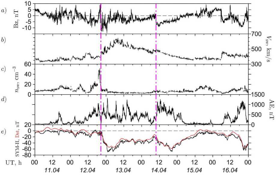
Figure 1. Interplanetary and geomagnetic conditions in the April 11–16, 2016 period: IMF B z ( a ); solar wind velocity V SW ( b ), solar wind density n SW ( c ), AE index ( d ), SYM-H (black line) and Dst (red line) indices ( e ). Vertical dash-dot lines indicate the time of the onset of storm main phases

increased to ~15:00 UT on April 15. A slight increase in substorm activity during the recovery phase of the second storm occurred from ~00:50 to ~2:25 UT on April 15, then AE returned to the quiet level. The entire recovery phase of the second storm lasted for ~18.5 hours, whereas that of the first storm did not end owing to the onset of the second storm.

Storms driven by CIR and/or subsequent high-speed streams typically recur every 27 days. For the April 12–15, 2016 storm, the recurrence took place on May 8–11, 2016 when the strongest geomagnetic storm of 2016 occurred (the main disturbance on May 8). Thus, these storms are classified as recurrent.

Next, we consider ionospheric disturbances generated by the April 12–15, 2016 geomagnetic storms. To better understand effects during the storms, we compare our results with those for the reference day of April 9, 2016, which is included in the list of the quietest days of the month — CK-days, International Q-days and D-days [].

2.    IONOSPHERIC DISTURBANCES

The impact of geomagnetic storms and substorms on the mid-latitude ionosphere, which manifests itself as electron density disturbances, has been studied using data from the set of scientific instruments located in Eastern Siberia. Measurements made with the vertical sounding ionosonde DPS-4 [Reinisch et al., 1997] , located in Irkutsk (52° N; 104° E), provided data on variations in the critical frequency f o F2 and F2 peak height h m F2. Ionograms were processed manually [Piggott, Rawer, 1972] .

Direct measurements of N e in an altitude range 150–600 km and of the vertical plasma drift velocity υ z were made with IISR (53° N; 103° E) [Zherebtsov et al. , 2002; Potekhin et al., 2009] . Methods for calculating N e and υ z drift from radar data are described in [Alsatkin et al., 2009; Shcherbakov et al., 2015] .

The paper also analyzes data on TEC variations from the dual-frequency GNSS receivers included in the International GNSS Service Network (IGS) [Dow et al., 2009] : IRKJ, IRKM (Irkutsk, 52° N; 104° E) and BADG (Badary, 51° N; 102° E).

As a criterion for evaluating the intensity of TEC variations we utilized the Rate of TEC Index ( ROTI ), which is a dispersion of TEC change rate [Pi et al., 1997]. ROTI series were averaged in a 5 min range. To account for the dependence of this index on elevation θ and to reduce all data to quasi-vertical values, we applied function M (ε) (for more detail, see [Sanz et al., 2013] ). This yielded the Along Arc TEC Rate ( AATR ) [Juan et al., 2018]. The time resolution of AATR corresponds to that of ROTI series.

We used GNSS data to analyze the dynamics of TEC noise spikes. To calculate this parameter from initial TEC series, we removed the trend to eliminate the effects of satellite motion and cut elevation series (θ ≥ 30º). Then we calculated the second TEC derivative, thus eliminating slow variations (seasonal, diurnal, tidal, etc.). As a result, there is only additive white Gaussian noise. The noise outside the 3σ threshold is considered to be the noise spikes.

Note that the local time in Irkutsk LT=UT+7.

Figure 2 shows f o F2 and h m F2 variations as derived from ionosonde measurements in Irkutsk on April 11–16,

2016 against the dynamics of these parameters on the reference day. Figure 3 shows altitude-temporal distributions of N e at 150–600 km ( a ), vertical plasma drift velocity variations υ z at 300 km (black line) and 350 km (red line) ( b ), and dynamics of ion ( c ) and electron ( d ) temperatures on April 11–15, 2016 from IISR data. The time resolution of υ z and temperature is 5 min; of all other parameters, 15 min.

During the period of high substorm activity on April 12, we observed an increase in f o F2 as compared to values on the reference day (Figure 2, a ), which was >1 MHz before the main phase of the first storms. After the beginning of the main phase and within 24 hours on April 13 there was a decrease in f o F2, followed by a slight increase in h m F2 (by ~20 km). In the altitude-temporal distributions of N e according to the IISR data, on April 13 there was also a pronounced decrease in N e by (1÷2)10⁵ cm^–3 (Figure 3, a ). In this case, the behavior of the vertical plasma drift differed from the quiet diurnal variation. From ~20:00 UT, ionospheric plasma rapidly drifted downward with a velocity up to 35 m/s at 300 km and with a velocity up to 25 m/s at 350 km (two times faster than under quiet conditions). This downward plasma drift was observed until ~00:00 UT (Figure 3, b ). Note that from ~10:00 UT on April 13 to ~ 01:00 UT on April 14, ionograms showed the F-spread effect (Figure 4, a ) indicating the presence of large-scale ionospheric irregularities.

The most significant amplitude ionospheric variations were recorded during the onset of the main phase of the second storm. Figure 2 shows that after ~09:40 UT there was a stepwise increase in f o F2 by ~3 MHz relative to the quiet level. As derived from radar data, the increase in N e was observed from 200 to 400 km, the maximum N e at 300 km was 9.2·10⁵ cm^–3, exceeding that for the reference day by 1.5 times (Figure 3, a ). At the same time, there was a positive jump in the plasma drift velocity.

With further development of the storm from 16:45 UT, the positive disturbance of foF2 became negative, and from ~20:00 UT after the minimum of foF2≈2.2 MHz reflections disappeared on ionograms, i.e. an intense absorption (blackout) began. The foF2 and Ne values significantly lower than those on the quiet day were observed throughout the recovery phase of the April 15 storm, whereas the near-noon maximum disappeared in the diurnal variation of Ne (Figure 2, a). The foF2 values were also low on April 16. The intensity of the negative ionospheric response was higher than that for the first storm, up to 2 MHz in foF2. The foF2 negative disturbance occurred with an increase in hmF2 to +55 km relative to the reference day (Figure 2, b). Note also that in the evening and night hours on April 14–15, plasma drift velocities were predominantly negative (Figure 3, b), and the modulus υz reached ~32 m/s, which is not typical of quiet conditions [Altadill et al., 2007] .

Ion T i and electron T e temperatures (Figure 3, c , d ) at different heights were obtained from IISR data, using the technique described in [Tashlykov et al., 2018] . T e hardly deviated from its quiet diurnal variation during the April 12–15, 2016 geomagnetic storms (Figure 3, d ). For ions, a temperature rose during the recovery phase of the storms on April 13 and 15 (Figure 3, c ). For the second storm, the positive deviation is more pronounced (up to 200 K between ~00:00 and 15:00 UT on April 15 relative to the quiet day on April 11).

Variations in the spatial averaged AATR for IRKJ, IRKM, and BADG reflect variations in the intensity of small-scale ionospheric irregularities in this region. Before the onset of the first storm, AATR was at the level of the reference day. It started increasing during the main phase of the first storm on April 13, and at ~4:45 UT (minimum SYM-H ) there was a sharp jump in AATR (Figure 4, b ). Then, several other AATR increases were observed. During the second storm, the jumps were recorded at the beginning of the main phase (~10:00 UT on April 14) and after maximum N e (Figure 3, a ) from ~12:00 to 14:00 UT. The quieter behavior of the second

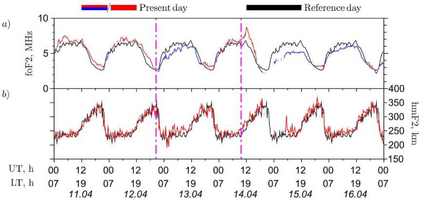
Figure2. Variations in F2-layer parameters on April 11–16, 2016: the critical frequency f o F2 higher (red line) and lower (blue line) than values on the reference day (black line) ( a ); the F2 peak height h m F2 (red line) and values on the reference day (black line) ( b )

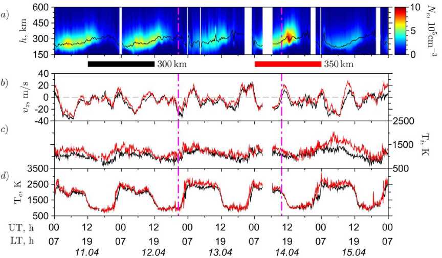
Figure 3. Variations of ionospheric parameters on April 11–15, 2016, as derived from IISR data: the electron density N e at 150–600 km in increments of 10 km and the height of maximum electron density (black line) ( a ); vertical plasma drift velocity υ z ( b ); ion temperature T i ( c ); electron temperature T e at 300 km (black line) and 350 km (red line) ( d )

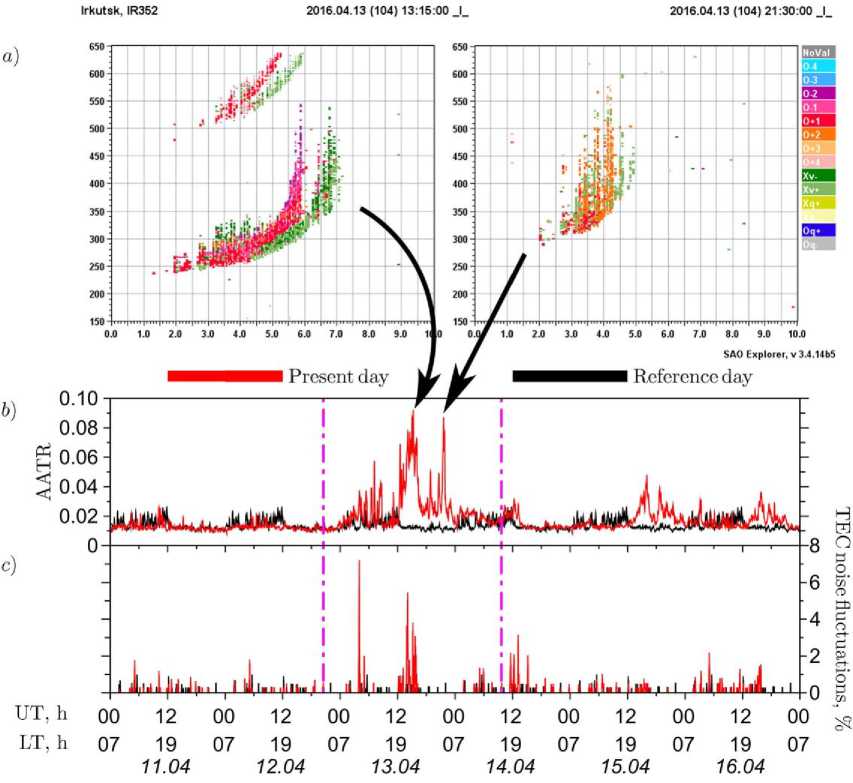
Figure 4. Examples of vertical sounding ionograms with F-spread effect ( a ) at 13:15 UT (left) and 21:30 UT (right) on April 13. Variations in AATR ( b ) and TEC noise spikes ( c ) on April 11–16, 2016 (red line) against the dynamics of these parameters on the reference day (black line)

storm also manifested itself in the absence of strong fluctuations of AATR during the recovery phase. In turn, the recovery phase during the first storm stands out as having strong disturbances of AATR whose values exceed those for the reference day 6–9 times. These disturbances began at ~12:00 UT on April 13 and reached extreme values by ~16:30 UT, and then started decreasing; during this period AATR values were about two times higher than those on the reference day (comparable to the disturbances during the main phase). Two more sharp jumps of AATR to extremely high values occurred at ~20:30 and ~21:30 UT. The constant excess over the level of the reference day lasted until ~4:00 UT on April 14. This interval is close to the period of F-spread observation on ionograms (Figure 4, a ).

TEC noise spikes indicate the presence of small-scale ionospheric irregularities, which affect the GNSS signal [Demyanov, Yasukevich, 2014; Demyanov et al., 2019] . By analyzing TEC noise data for April 12–15, 2016, averaged at each time point for IRKJ, IRKM, and BADG receivers, and considering their deviations from those for the reference day, we determined moments of the greatest noise spikes (Figure 4, c ). The obtained TEC spikes distribution correlates well with AATR variations, in particular in the interval of extremely high AATR from ~04:00 to ~16:30 UT on April 13 in the recovery phase of the first storm (Figure 4, b ). Higher noise spikes were also recorded on April 14 during the second storm. Thus, the noise spikes and extremely high AATR indicate the intensification of small-scale ionospheric disturbances caused by disturbed geomagnetic conditions and high substorm activity. The percentage of noise spikes increased, on average, 2–2.5 times relative to the reference day.

3.    MANIFESTATIONSIN THE OPTICAL RANGE

Of particular interest is the atmospheric response to geomagnetic disturbances manifesting themselves as airglows. We have studied the dynamics of 557.7 and 630 nm atomic oxygen emission intensities. Maxima of these emissions in the atmosphere are located at heights of 97 and 270 km respectively. The most intense emission generally occurs at the 630 nm wavelength, which also directly depends on Dst [Mikhalev, 2013] . This emission is often regarded as an indicator of changes in N e and dynamics of the upper atmosphere during mid-latitude airglows. At the same time, there is no consensus about the dependence of the 557.7 nm emission intensity on the geomagnetic activity level [Leonovich et al., 2012] . As a control parameter we considered the 470 nm airglow intensity.

The emission intensity was studied using a wide-angle highly sensitive camera FILIN-1C installed in the village of Tory (52° N; 103° E) with an exposure of 300 s. In the period of interest on April 12–15, 2016, the camera worked every day from ~13:00 to ~21:00 UT, but data to ~14:00 UT and after ~20:00 UT was ignored because of strong influence of sunset/sunrise. Thus, for the study we used data on April 13 (the recovery phase of the first storm) and April 14 (the main phase of the second storm).

Note that in the said period there were dense clouds and a high position of the Moon. These factors have an equal effect on the emission intensity at all wavelengths, therefore they do not hinder the identification of emission intensity variations at one wavelength relative to the other.

To study the emission variations, we calculated the ratio of differences between intensities of the 630 nm emission and the other two (557.7 and ~470 nm) to the 630 nm emission intensity. We found no significant deviations in comparison with the reference day of April 13, although there were some fluctuations in the 630 nm emission from ~17:00 to 18:00 UT (Figure 5, a ). Disturbances on April 14 began after ~18:00 UT, and at ~19:30 UT a peak increase in the 630 nm emission intensity relative to the other two occurred. The 630 nm emission intensity was high until the end of observations on April 14 (Figure 5, b ).

Taking into account that these storms are minor, the 630 nm emission intensity increase is most likely to be caused by collisions between oxygen atoms and thermal electrons of the ionosphere or dissociative recombination [Tashchilin, Leonovich, 2016] .

The low intensity of the storms may also be the reason why we have not recorded the increase in the 557.7 nm emission intensity, normally observed during strong geomagnetic storms.

CONCLUSION

Using data from a set of radiophysical and optical instruments, we have studied variations in different ionospheric parameters during two geomagnetic storms on April 12–15, 2016.

We have shown that these storms are classified as recurrent without sudden commencement. Solar sources of such storms are coronal holes and their associated highspeed plasma streams.

While both the storms were relatively weak, there was a pronounced ionospheric response to these disturbances. During the main phase of these storms, we observed negative disturbances of the electron density N e and critical frequency f o F2. For the second storm, the amplitude of the negative response was higher, a decrease in f o F2 was larger than 30 % relative to the quiet level. This can be explained by the fact that the second storm occurred during the recovery phase of the first one when ionospheric plasma was already disturbed. The f o F2 negative disturbance was accompanied by an increase in the F2 peak height. We also recorded predominantly negative plasma drift velocities in the evening and night, which differs from the characteristic behavior under quiet conditions. After the main phase of the second storm, the ion temperature rose by 200 K relative to the quiet day too, indicating a general increase in the thermospheric temperature. The increase in the thermospheric temperature during geomagnetic storms produces a negative response in the mid-latitude ionosphere [Klimenko et al., 2017] . During the main phase of the second storm, we also detected a peak increase in the 630 nm emission intensity in the atmosphere.

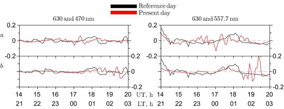
Figure 5. Airglow disturbances on April 13 ( a ) and April 14 ( b ): the ratio of difference between 630 and 557.7 nm (right), 630 and 470 nm (left) emission intensities to the 630 nm emission intensity (red line) against the same values on the reference day (black line)

An interesting feature of the second storm was a 1.5-fold abrupt increase in N e during the early main phase of the storm. This positive disturbance was observed for ~ 7 hours in the daytime and was accompanied by significant positive vertical plasma drift velocities, atypical for this time of day.

During the period of interest, we recorded abrupt increases in AATR and TEC noise spikes, associated with the development of small-scale irregularities. These increases had great intensity during the first storm with F-spread on ionograms but were more frequent during the second storm. On average, the percentage of noise spikes increased 2–2.5 times relative to the reference day.

We thank Yasyukevich Yu.V., Vesnin A.M., Tash-lykov V.P., Vasiliev R.V., and Ratovsky K.G. for advice and assistance with data. The data on geomagnetic indices used in this paper was taken from the site of World Data Center for Geomagnetism (WDC for Geomagnetism, . We used data from the Unique Research Facility Irkutsk Incoherent Scatter Radar . Irkutsk ionosonde data were obtained using the equipment of Center for Common Use «Angara» []. AATR values were calculated using the System for the Ionosphere Monitoring and Researching from GNSS [Yasyukevich et al., 2018]. The work was performed with budgetary funding of Basic Research program II.16 (analysis of storm dynamics, IISR data, and optical measurements) and of RF President grant No. MK-3265.2019.5 (analysis of AATR and TEC noise variations).