Weight assignment algorithms for designing fully connected neural network

Author: Aarti M. Karande, D. R. Kalbande
Journal: International Journal of Intelligent Systems and Applications @ijisa
Article in issue: 6 vol.10, 2018.
Free access
Soft computing is used to solve the problems where input data is incomplete or imprecise. This paper demonstrate designing fully connected neural network system using four different weight calculation algorithms. Input data for weight calculation is constructed in the matrix format based on the pairwise comparison of input constraints. This comparison is performed using saaty’s method. This input matrix helps to build judgment between several individuals, forming a single judgment. Algorithm considered here are Geometric average mean, Linear algebra calculation, Successive matrix squaring method, and analytical hierarchical processing method. Based on the quality parameter of performance, it is observed that analytical hierarchical processing is the most promising mathematical method for finding appropriate weight. Analytical hierarchical processing works on structuration of the problem into sub problems, Hence it the most prominent method for weight calculation in fully connected NN.
Soft Computing, Neural Network, Saaty’s Method, Analytical Hierarchical Processing, Exact Linear Algebra Calculation, Geometric Average Approximation, Successive Matrix Squaring
Short address: https://sciup.org/15016501
IDR: 15016501 | DOI: 10.5815/ijisa.2018.06.08
Text of the scientific article Weight assignment algorithms for designing fully connected neural network
Published Online June 2018 in MECS
Finding a solution to a real time problem is difficult as it may depend on the type of problem, sensitivity of the problem, and type of solution expected. Soft computing approach helps to find a solution in unpredictable situation. Neural network (NN) is one of the techniques of the soft techniques. NN requires weights to be assigned among neurons for calculating result. This paper discusses 4 different algorithms for calculating weights based on input given to the neurons. This paper also compares stated algorithm with an example.
-
A. Soft Computing Approach
Using computer technology, a process which completes a task is called as computing. Computing is classified into two types. First is Hard computing, i.e., conventional computing concept which uses the available analytical calculation model. Second is Soft computing, which works as a tolerant of imprecision, uncertainty, partial truth, and approximation. [28] It describes and transforms information such as theory, analysis, design, efficiency, implementation, and application as that of the human mind. [1] [25] The main characteristic of soft computing is its intrinsic capability to create hybrid systems based on a (loose or tight) integration of the constituent technologies. [5] This integration combines unclear domain knowledge and empirical data to develop flexible computing tools and to solve complex problems based on the reasoning. [25][8][16] Soft computing is more oriented towards the analysis and design of intelligent systems.
Soft computing (SC) has a different technique like neural networks, fuzzy logic, genetic algorithm, swarm optimisation and their hybrid combination. [9] SC has strong learning and cognitive ability and good tolerance of uncertainty and imprecision. SC techniques derive their power of generalisation generating output from previously unseen or learned inputs based on approximation. [25] Soft Computing algorithms are used for real time understandable application.
Advantages of Soft Computing can be listed as
-
• Nonlinear problems can be solved using SC;
-
• It works in human knowledge areas such as cognition, recognition, understanding, learning, and computing.
-
• Intelligent systems such as autonomous self-tuning systems, and automated designed systems can be constructed using SC.
-
II. Structure of the Neural Network
-
A. Artificial Neural Network
The artificial neural network is one of the main techniques of soft computing. [20] [23] [5] NN are nonlinear predictive models that learn through experience and training. NN models are non-parametric models. [17] NN are universal function approximators. [19] NN and statistical approaches differ in assumptions about the statistical distribution or properties of data. NNs gives much accurate when modelling complex data.
NN system will adapt to the input environment. [12] It will produce the output depending upon its input. The output of one node can be the input of another node. The final output depends on the complex interaction among all the nodes. [32] [5] A characteristic of NN depends on its structure, the connection strength between neurons (i.e. synaptic weights between neurons), i/p and o/p node properties, and error calculation rules. The power of neural computations depends on connecting neurons in the network. [30] NNs are potentially useful for understanding the complex relationships between input and output. NN can perform data analysis for imprecise and incomplete input.
The working of a neural network is determined by its activation functions, learning rule, and based on the connection of neurons itself. [26] During training, the inter-unit connections are optimised till the error in predictions is minimised or the network reaches the specified level of accuracy. The network is trained and tested with input pattern.
There are three major steps of execution in the NN
-
1. Pre-processing: It is the learning process based on the information environment of the system. In this phase, required input and output information are collected. These data are first normalised or scaled to reduce noise. During this process, NN reduces the error between expected value and calculated output value by adjusting the weights between neurons. Weights are calculated or modified based on the learning rules or states of the processing elements. Preprocessing may calculate the number of turns used to train NN.
-
2. Learning algorithm: It gives the sets of instruction in the NN for modifying the network weights as per the learning rule. It builts a variety of NN that could be used to capture the relationships between the inputs and outputs. The working of this step depends on the information environment.
-
3. Post Processing: This process is done after understanding, learning algorithm, learning capacity of the network, the complexity of the network, and time complexity of the network. This process generates patterns of weights to determine any arbitrary input. Different trading strategies are applied to maximise the capability of the NN prediction.
Training a NN is adapting its input values so that the model exhibits the desired computational output. [20] Types of learning methods are
-
1. Supervised learning where i/p pattern given to the network knows its output in the learning process.
-
2. Unsupervised learning, where i/p pattern does not
have guidelines or target output in the learning process.
NN can learn new associations, new functional dependencies and new patterns based on the input or output values. [24] NN can automatically adjust their weights to optimise their input behaviours. [27]
-
B. Features of neural network
-
• They are Non-Linear, Fault Tolerant. [32][15]
-
• NNs are less sensitive to noise, chaotic components and heavy tails better than most of the other methods
-
• This model can be easily and quickly updated. [20][10]
-
• NN can determine complex function approximations, classifications, auto associations, etc. [24][5]
-
• It shows the cause-effect relationship between independent and dependent variables with processing speed.
-
• NN acts as a black box and automatically predict output for the user. [1][22]
-
C. Applications of the NN
-
• NN can be used in a pattern or trend recognition of data, classification, signal processing,
unsupervised clustering, visualisation of complex data, data compression, controlling problems and image processing. [16][23] It correctly handles incomplete patterns of recognising information. [15][20][32]
-
• It can also be used in prediction or forecasting areas such as Sales forecasting, Industrial process control, Customer research, Data validation, Risk management and Target marketing and so on. [2][17][7]
-
• Some more application domains are Statistics and Economics, Insurance and Finance, Space, Automotive and Correspondence, Medicine marketing, manufacturing, operations, information systems, and so on. [8]
-
• It can be used to identify fault-prone modules in the software; to learn index rules and adaptation functions for communication network;
-
• It is used to identify faults in switching systems; act as a preprocessor for a fault diagnosis expert system.
-
• Complex NN can work as intelligent hybrid systems in the applications such as process control, engineering design, financial trading, credit evaluation, medical diagnosis, and a cognitive simulation.
-
D. Disadvantages of the NN
-
• Even though this network is easy to over fit, but training rules are hard to extract and to understand.
-
• This network works in a parallel but it is difficult to work in distributed information processing
nature.
-
E. Fully Connected Neural Network
In fully connected NN, all neurons are connected to each and every neuron. Hence this structure is having high strength for fault tolerance. This connected structure needs to assign weights among all nodes. The NN has the ability to capture the nonlinear patterns of the failure process by learning from the failure data, i.e. to learn the network so that to develop its own internal model of the failure process. [6][15] Fully connected NN has a simple structure and it is relatively easy to implement. Its operating principles and characteristics can be extended to other types of networks, even if some of its connections are missing. [33]A standard fully-connected neural network of L neurons has three types of layers:
-
• An input layer (u0 i ) whose values are fixed by the input data.
-
• Hidden layers (u i l ) whose values are derived from the previous layers.
-
• An output layer (u i L ) whose values are derived from the last hidden layer.
The neural network learns by adjusting a set of weights, wℓi j , where wℓi j is the weight from some unit u i l 's output to some other unit u i l+1. [44] Running the network consists of two-pass circulations:
-
1) Forward pass: the outputs are calculated and the error at the output units are also calculated based on following steps;
-
1. Compute activations for layers with inputs using equation (1) :
-
2. Compute inputs for the next layer from these activations using equation (2):
-
3. Repeat steps (1) and (2) until you reach the output layer, and know values of yℓi.
yℓ i = σ (xℓ i ) + Iℓ i (1)
xℓ i =∑ j wℓ-1 ji .y ℓ-1 j (2)
With the previously listed functions and effectively means, error must be computed and summed. NN error E (yL) function can be a binary cross-entropy or sum of squared residuals. Still, derivative dE (yL) / dyLi depend only on yLi.
-
2) Back-ward pass: Based on the output unit, error is
used to alter the weights on the output units. Then the error at the hidden nodes is calculated, and the weights of the hidden nodes altered using these values. This procedure is repeated till the error is at a low enough level. The purpose of computing the error is to optimise the weights so that to minimise the error in the next level of phase. In order to use gradient descent to train NN, It is required to compute the derivative of the error with respect to each weight. Using the chain rule using equation (3),
∂E/∂wℓ ij = ∂E/∂xℓ+1 j . ∂ xℓ+1 j /∂wℓ ij (3)
The equation for forward propagation (xℓi=∑jwℓ-1 j i.yℓ-1 j ), the partial with respect to any given weight is just the activation from its origin neuron. Thus, the chain rule above becomes as shown in equation (4)
∂E/∂wℓ ij =yℓ i .∂E/∂xℓ+1 j
Input layer
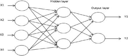
Fig.1. Structure of Fully connected Neural Network
-
III. Weight Calculation Algorithm For Neural Network
The Neural network is trained based on the connection of input to output layers with hidden layer. Weight is assigned to each connection based on its importance of connection. Mathematical methods can be used to assign weights to neuron link. This paper shows mathematical models for assigning weights to fully connected NN using saaty’s method. The weights of NN are the most adjustable and important parameters of NN. The weighted sum of the inputs constitutes the activation of the neuron. The activation function produces output of the NN.
-
A. Saaty’s Method for Comparison Matrix
Saaty developed an algorithm finding the importance of input depending on pairwise comparison among inputs forming priority matrix or comparison matrix. [4] Comparison matrix gives a ranking of inputs that indicates an order of favouritism among them. Ordering should reflect cardinal preference indicated by the ratios of value. [29] A priority matrix need to reproduce itself on a ratio scale based on the strength of preferences.
Priority matrix should be invariant under the hierarchic level of composition. The matrix is formed as per the suggestion from the experts for pairwise comparison of inputs based on constraints given in the table 1. Suppose we compare input k with input l. The priority matrix has much less validity for an arbitrary positive reciprocal matrix B = (bkl) than for a consistent matrix. For assigning values bkl and blk using equation (5)
^ bk = 1 for all k = l
^ b ik = 1 / b ki (5)
where b kl = intensity of importance of input k over l .
Thus we obtain B= [bkl] for k * l . Values need to be within range {1…9} forming a square matrix. This matrix is evaluted for computing eigenvector using different mathematical model.
Table 1. Pairwise comparison for attribute importance
|
Intensity of Importance |
Definition |
Explanation |
|
1 |
Equal Importance |
If both input data is having equal importance |
|
3 |
Moderate Importance |
If first data is slightly favor one activity over another data |
|
5 |
Strong Importance |
If first data is strongly favor one activity over another data |
|
7 |
Very Strong demonstrating importance |
If first data is favored very strongly over another its control demonstrated in practice |
|
9 |
Extreme Importance |
If first data evidence favoring one activity over another data is of the highest possible order |
The pairwise comparison matrix is formed, considering the relative significance of rows with that of columns. The matrix is builds based on the reciprocal property. This matrix helps to build judgment of several individuals’ input combining it into a single judgment. The normalised eigenvector of the comparison matrix gives the relative importance of the input. The normalised eigenvector is termed as weights for NN with respect to the input comparison.
-
B. Different weight Calculation Algorithm
-
B.1 Geometric Average Approximation (GA)
-
The Geometric Average method (GA) is rigidly defined only for the inputs. Different user will also find the same result in storing data. This method works as per the rate of return that connects the starting and ending values if it is considered in all periods of calculation. It works on relative measure of data. It gives less importance to large items and more to small ones. This method works as an algebraic treatment for defining increase or decrease in the rate of input data. [33] This method helps to find combined geometric means of the series. This method utilises measurement methods for finding the investment of returns as per the input matrix.
Input: matrix A[i] [i] Output: weight W[i]
Begin
B[i] =1, sum=0
For each row m= 1 to i
For each column n=1 to j
B[m] = A[m] [n]* B[m]
For each row m= 1 to i
C[m] = power (B[m], 1/j)
Sum = sum + C[m]
For each row m=1 to i
W[m] = C[m]/sum
End
Algorithm 1: Geometric Average Approximation
Disadvantage of the geometric average method is that it is not widely used. If any of the input value is zero or negative, then this method becomes indeterminate. This method is not suitable for open-end class interval of the data.
-
B.2 Exact Linear Algebra Calculation (EA)
Exact linear algebra (EA) includes calculating a solution of linear equations with input as precise value, integers modulo, a prime number, residues modulo, or a minimum polynomial. This method is used for finding matrix’s rank, its determinant, its minimal polynomial, and its rational canonical form. [10]
Input: A[i] [j]
Output: weight W[i]
Begin
B[i] =0, C[i] [j] =0; sum[i] =0
For each column n= 1 to j
For each row m=1 to i
B[n] = A[m] [n] + B[n]
For each row m= 1 to i
For each column n= 1 to j
C[n] [m] = A[i] [j] / B[n]
For each row m= 1 to i
For each column n= 1 to j
Sum[m] = sum[m] +C[m] [n] W[m] = sum[m]/j
End
Algorithm 2: Exact Linear Algebra Calculation
Disadvantage of the Exact Linear Algebra Calculation method is that it could easily be unstable for computing large determinant. Also, it does not find approximate solutions as that of the least square method. [14]
-
B.3 Successive Matrix Squaring (SMS)
The Successive matrix squaring algorithm (SMS) is used for calculating the generalised inverse of a given pairwise comparison matrix as A Є Cm×n. [25] SMS is a deterministic iterative algorithm for finding matrix inversion based on a continuous repetitive matrix squaring technique. [21] SMS specifies generalised inverse with the specified range. SMS works on the policy for displacement rank with given specified ranges. [13] Parallel matrix generated at the end of each calculation, changes the elements of the original matrix. [18]This method is simple multiplication of matrix with itself a number of times, and result of calculations are not stored at the end of each cycle. This method takes more calculation time on typical parallel architectures. [31]
Input: A[i] [j]
Output: weight W[i]
Begin
//Phase 1:
B[i] =0, C[i] [j] =0; sum[i] =0
For each row m=1 to i
For each column n= 1 to j
B[m] = A[m] [n] + B[m]
For each row m= 1 to i
Sum = Sum + B[m]
For each row m= 1 to i
W1 [m] = B[m]/ sum
//Phase 2:
B[i] =0, C[i] [j] =0; sum[i] =0
For each row m=1 to i
For each column n= 1 to j
A1 [m] [n] = A[m] [n] + A[n] [m]
For each row m=1 to i
For each column n= 1 to j
B[m] = A1 [m] [n] + B[m]
For each row m= 1 to i
Sum = Sum + B[m]
For each row m= 1 to i
W2 [m] = B[m]/ sum
//Phase 3:
For each row m= 1 to i
W[m] = w1 [m]-w2 [m]
For each row m= 1 to i
If w[m]>0.01
For each row m = 1 to i
W [m] =w1 [m] End
Algorithm 3: Successive Matrix Squaring
A disadvantage of the SMS method is its matrix size (m + n). In the case of m ≈ n, it will perform almost ≈ (2n)3 operations on the matrix. [13]
-
B.4 Analytical Hierarchical Processing (AHP)
The Analytical Hierarchical Processing (AHP) divides the problem into the order of a set of sub problems. This makes the problem easy to solve and easy for calculation as per the sub problems. [11] Normalised eigenvector is calculated on the basis of the relative intensity of the input vector. The normalised eigenvector is termed as weights with respect to the input vector. Consistency index (CI) of this matrix is compared with that of the relative index (RI) of the matrix. Consistency ratio CR = CI / RI is calculated. If calculated consistency ration CR does not match with the required level (i.e. greater than 0.1), then pairwise comparisons matrix values are reentered. [27] AHP is used for setting priorities of input criteria. This method of pairwise comparison is very straightforward and convenient. It is also used in subjective and objective evaluation for real time problem. It is flexible and able to check inconsistencies in the input data. AHP has been applied in decision-making scenarios such as a selection of one alternative from a set of alternatives, determining the relative merit of a set of alternatives, finding the best combination of alternatives, subject to a variety of constraints, Benchmarking of processes or systems with other in quality management.
Input: A[i] [j]
Output: weight W[i]
Begin
B[i] =0, C[i][j]=0; sum[i]=0; CI=0
For each column n= 1 to j
For each row m=1 to i
B[n] = A[m][n]+ B[n]
For each row m= 1 to i
For each column n= 1 to j
C[m]= C[m]+ (A[m][n] / B[n])
For each row m= 1 to i
For each column n= 1 to j C[m]= C[m]/j For each row m= 1 to i
For each column n= 1 to j
W[m]= C[m] * A[m][n]
For each row m = 1 to i // for consistency index Sum = w[m] +sum CI = (sum – i) / (i-1) If CI <0.1
Weight are considered
Else
Change weight
End
Algorithm 4: Analytical Hierarchical Processing
AHP has a disadvantage for its number of pairwise comparisons. [4] It is equal to (n*(n-1)/2) comparisons for n number of inputs. This method is lengthy and timeconsuming. It has an artificial limitation to use the scale of the 9 point only as per the saaty’s method. [24] Comparison between all methods
-
C. Steps for Weight Calculation Method
To compare weighting algorithm for fully connected NN, following step is performed
Step 1: Construct a neural network pairwise matrix for input, hidden and output layers.
Step 2: Pairwise comparison matrix based on saaty’s concept is built for the input layer to hidden layer and for hidden layers to the output layer. For matrix, number of input node will work as rows and the number of hidden layers will work as columns. Same steps of executions are followed for hidden layer to the output layer. (If hidden layer is not present, then a comparison matrix is built between input layer and output layer)
Step 3: Find eigen vector for giving pairwise matrix. (or for hidden layer if applicable).
Table 2. Comparison Of Weighting Algorithm
|
GA |
EL |
SMS |
AHP |
|
Working |
|||
|
It is rigidly defined |
It computes an exact solution work on matrix. It performs computing like rank, determinant, characteristic and minimal polynomial |
It approximate the weighted generalised inverse, Simply repeat the squaring operation k times so no need to save the data. |
Sets the priority of the input criteria as per the pair wise comparison. |
|
Usage |
|||
|
Used to get a rate of investment that connects the starting and ending asset values |
Used in converting a large number of problems to matrix. |
Used to find various outer inverses with given ranges and null spaces |
more easily comprehended , divided and subjectively evaluated |
|
Disadvantage |
|||
|
Becomes indetermin ate if any value in the given set is zero or negative. |
Unstable for computing large determinant. |
Time-consuming operation on typical parallel architecture For matrix of size m*n, if m ≈ n then it perform almost ≈(2n) operation |
Numbers of pair wise comparisons are (n (n-1)/2) It is a lengthy task. Limited to the use of 9 point scale. |
-
IV. Mesuring Business Process Criticality Using Neural Network Using Weighting Algorithm
To measure usage of weighting algorithm, I have developed a JAVA based tool for measuring business process criticality of an enterprise solution. This tool calculates criticality of the process by assigning each neuron with value as per the type of architecture level process is working, and as per the type of process. Architecture levels are Business level (BL), Information level(IL), Data level(DL), Application level (AL) and infrastructure level(TL). Process type is Management process (MP), the Core process (CP), Enabling process (EP), and Enhancign process(EEP). Using saaty’s pairwise comparion, a matrix is constructed for architectural level vs process type as shown in table 4. For simplicity, fully connected NN of five neurons is considered for a problem as shown in the figure 2.
-
A. Construction of 5 neuron Fully connected NN
A neural network of 5 neurons are constructed as shown in the figure 2. As shown in the table 4, values are forwarded to NN
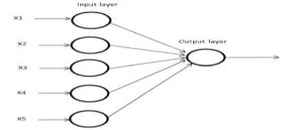
Fig.2. Structure of 5 neuron fully connected NN
Table 3. Pairwise Comparison For 5 Input Nodes
|
BL |
IL |
DL |
AL |
TL |
|
|
MP |
1 |
5 |
3 |
7 |
6 |
|
CP |
0.2 |
1 |
0.33 |
5 |
3 |
|
EP |
0.33 |
3 |
1 |
6 |
3 |
|
EEP |
0.14 |
0.2 |
0.17 |
1 |
0.33 |
-
B. Using Geometric Average Approximation
This is the simplest method for finding eigen value using following formula shown in using equation (6)
F = ((multiplication of row value) 1/no. of element / sum of all
(multiplication of row value))(6)
Table 4. Weight Calculation Using GA Method
|
BL |
IL |
DL |
AL |
TL |
F |
Weight |
|
|
MP |
1 |
5 |
3 |
7 |
6 |
3.63 |
0.50 |
|
CP |
0.2 |
1 |
0.33 |
5 |
3 |
1.00 |
0.08 |
|
EP |
0.33 |
3 |
1 |
6 |
3 |
1.78 |
0.15 |
|
MP |
0.14 |
0.2 |
0.17 |
1 |
0.33 |
0.28 |
0.02 |
|
Sum |
0.67 |
4.2 |
1.5 |
12 |
6.33 |
0.67 |
C. Using Exact Linear Algebra
This method gives new matrix based on each row calculation. For each row, for each cell find value as shown in equation (7)
= Cell value / sum of column values(7)
Find the weight matrix using equation (7)
Weight matrix = Sum of the row value / no. of the element in the row(8)
Table 5. Weight Calculation Using El Method
|
BL |
IL |
DL |
AL |
TL |
Weight |
|
|
MP |
1 |
5 |
3 |
7 |
6 |
0.49 |
|
CP |
0.2 |
1 |
0.33 |
5 |
3 |
0.14 |
|
EP |
0.33 |
3 |
1 |
6 |
3 |
0.27 |
|
MP |
0.14 |
0.2 |
0.17 |
1 |
0.33 |
0.02 |
|
Sum |
0.67 |
4.2 |
1.5 |
12 |
6.33 |
-
D. Using Square matrix multiplication
This method calculates the new matrix by multiplying itself, i.e. Matrix * Matrix. Calculate eigen values based on the formula, the sum of row wise data divided by the sum of column wise value.
Perform the same step, finding new matrix with matrix multiplication with new values. Using the same steps find new weights. Find the difference between two weights. If the difference is <0.01 then new calculated weights will be final weights.
Table 6. Weight Calculation– Calculation 1
|
BL |
IL |
DL |
AL |
TL |
F |
Wt |
|
|
MP |
4.99 |
22.3 |
10.8 |
75 |
38.31 |
151.50 |
0.50 |
|
CP |
1.71 |
4.98 |
3.1 |
22.38 |
9.84 |
42.02 |
0.14 |
|
EP |
2.61 |
9.84 |
8.49 |
38.31 |
18.96 |
78.21 |
0.26 |
|
MP |
0.43 |
1.71 |
0.93 |
4.99 |
2.61 |
10.69 |
0.04 |
|
Sum |
130.92 |
Table 7. Weight Calculation– Calculation 2
|
BL |
IL |
DL |
AL |
TL |
F |
Wt1 |
|
|
MP |
159.84 |
577.28 |
353.88 |
2078.39 |
1003.45 |
4172.84 |
0.49 |
|
CP |
44.10 |
178.74 |
98.88 |
577.28 |
281.14 |
1180.14 |
0.14 |
|
EP |
86.38 |
303.31 |
200.56 |
1137.54 |
552.38 |
2280.17 |
0.27 |
|
EEP |
12.15 |
44.10 |
27.28 |
159.84 |
77.25 |
320.61 |
0.04 |
|
Sum |
3780.92 |
Step 4: find the difference between weights using equation (9)
Weight = weight 1 – weight 2 (9)
Table 8. Sms Method – Difference In Weight
|
Weight 1 |
Weight 2 |
Difference |
|
|
MP |
0.50 |
0.49 |
0.01 |
|
CP |
0.14 |
0.14 |
0.00 |
|
EP |
0.26 |
0.27 |
-0.01 |
|
EEP |
0.04 |
0.04 |
0.00 |
Repeat the step till difference between weight 1 and new weight 2 or so on is minimised. If yes, take new weight as the weight.
-
E. Using Analytical Hierarchical Processing
This method finds consistency index, if CI is > 0.1, considered value as input is assumed to be correct. Otherwise, reconsider the input value. Find the eigen value using the formula as shown in quation (10)
λmax = Sum (row value / sum of column)/ no. of element hence for given values λmax will be
λmax =( 5.53+5.22+5.55+5.08+5.06)/5= 5.29
Calculated consistency index will be
Consistency index = (λmax-n) / (n-1) => 0.0729
If CI is <0.1 so considered data is accepted. Hence calculated weight will be final weight.
Table 9. Weight Calculation Using AHP Method
|
BL |
IL |
DL |
AL |
TL |
F |
Wt |
|
|
MP |
1 |
5 |
3 |
7 |
6 |
0.49 |
5.53 |
|
CP |
0.2 |
1 |
0.33 |
5 |
3 |
0.15 |
5.22 |
|
EP |
0.33 |
3 |
1 |
6 |
3 |
0.24 |
5.55 |
|
MP |
0.14 |
0.2 |
0.17 |
1 |
0.33 |
0.04 |
5.08 |
|
Sum |
0.67 |
4.2 |
1.5 |
12 |
6.33 |
1.00 |
F. Comparison of All Methods for Weights
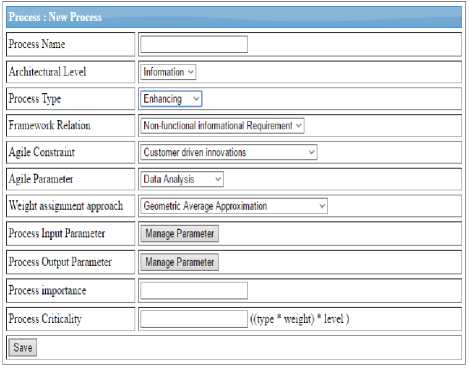
Fig.3. Screen shot of phase tool for weight assignment method
After analysis of all mathematical models for calculating weight for NN, AHP method is the most promising method. After understanding the advantages and disadvantages of methods, it is found that AHP is a most prominent method. Even though it is taking more time to calculate the answer, it works in a more systematical way.
Table 10. Comparison Of Weights
|
Input Node |
GA |
LA |
SMS |
AHP |
|
MP |
0.50 |
0.49 |
0.49 |
0.49 |
|
CP |
0.08 |
0.14 |
0.14 |
0.15 |
|
EP |
0.15 |
0.27 |
0.27 |
0.24 |
|
MP |
0.02 |
0.02 |
0.04 |
0.04 |
These algorithms are compared on the basis of the quality parameter such as speed, accuracy, and complexity of evaluation. These parameters are evaluated for measuring speed of execution, accuracy of the result and for the complexity of algorithmic calculation. A number of evaluation loops present in GA, LA and SMS are low compared to AHP. Based on the number of temporary storage, accuracy of result is calculated for AHP which gives accurate answer. For finding answers GA, LA and SMS are less complex compared to AHP. In case of complexity, calculation in AHP is more complex compared to another method. In AHP pairwise comparison of input is done in the structural way; AHP gives more accurate result.
-
V. Conclusion
Soft computing system works on repetitive observation and on adaptive methodology. Neural networks can attain and utilise stored data for finding real time solutions. NN work for tuning the problem. This paper helps to find the weight of NN’s neurons based on four different mathematical models. Even though these mathematical models are having their advantages and disadvantages still depending on the requirements of the system, a mathematical model can be selected for the fully connected neural network. These methods are compared for the quality parameters such as speed, accuracy and complexity. After evaluating a simple example, it is found that analytical hierarchical method is the best method for calculating weight of the neurons in the fully connected neural network. AHP considers input parameter comparsion in detail. AHP gives accurate result even though this method is time-consuming.
Future work
This mathematical model can be further applied to some more application of NN such as gaming theory, image processing, data analytics and so on to check their validity.
References Weight assignment algorithms for designing fully connected neural network
- Abraham and Baikunth Nath, (2000) “Hybrid Intelligent Systems: Review of a Decade of Research” Technical Report Series, 5/2000
- A.Maithili Dr R. Vasantha Kumari Mr S. Rajamanickam (2012) Neural Network towards Business Forecasting IOSR Journal of Engineering, pp: 831-836ISSN:2250-3021
- Angela Bower (July 2003) Soft Computing tessell A Support Services Plc Issue V1.R1.M0
- Ajith Abraham, Johnson Thomas, Marcin Paprzycki, Brent Doeksen,(2005)"Real Stock Trading Using Soft Computing Models", vol.02,pp.162-167,doi:10.1109/ITCC
- Anita Ahmad Kasim Retantyo Wardoyo and Agus Harjoko (2017) Batik Classification with Artificial Neural Network Based on Texture-Shape Feature of Main Ornament I.J. Intelligent Systems and Applications, 2017, 6, 55-65 DOI: 10.5815/ijisa.2017.06.06 Copyright © 2017 MECS I.J. Intelligent Systems and Applications, 2017, 6, 55-65
- Basheer M. Al-Maqaleh a , Abduhakeem A. Al-Mansou Fuad N. Al-Badani “Forecasting using Artificial Neural Network and Statistics Models” (2016) I.J. Education and Management Engineering, DOI:10.5815/ijeme.2016.03.03
- Dragan Z. Šaletic (2006) “On Further Development of Soft Computing, Some Trends in Computational Intelligence” SISY 4th Serbian-Hungarian Joint Symposium on Intelligent Systems
- Erich L. Kaltofen, Arne Storjohann “The Complexity of Computational Problems in Exact Linear Algebra” Encyclopaedia of Applied and Computational Mathematics, Bjorn Enquist, Mathematics of Computer Science, Discrete Mathematics,JohanHastad,field, Springer
- Ebru Ardil and Parvinder S. Sandhu (2010) “A soft computing approach for modelling of severity of faults in software systems” International Journal of Physical Sciences Vol.5 (2), pp.074-085,ISSN 1992-1950
- Ezhilarasi G and Dhavachelvan P (2010) “Effective Web Service Discovery Model Using Neural Network Approach” International Journal of Computer Theory and Engineering, Vol. 2, No. 5
- Geoff Coyle: Practical Strategy (2004) Open Access Material. AHP © Pearson Education Limited
- Prof. Dr. Hanan A. R. Akkar Firas R. Mahdi (2017) “Adaptive Path Tracking Mobile Robot Controller Based on Neural Networks and Novel Grass Root Optimization Algorithm” I.J. Intelligent Systems and Applications, 2017, 5, 1-9 DOI: 10.5815/ijisa.2017.05.01 MECS I.J. Intelligent Systems and Applications, 2017, 5, 1-9
- Lujuan Chen, E.V. Krishnamurthy, Iain Macleod (1994) Generalized matrix inversion and rank computation by successive matrix powering parallel Computing20-297-311
- Linear algebra: numerical methods. Version: Aug 12, 2000
- Kurhe A.B., Satonkar S.S., Khanale P.B. and Shinde Ashok (2011) “Soft Computing and its Applications BIOINFO Soft Computing” Volume 1, Issue 1, pp-05-07
- Kate A. Smith, Jatinder N.D. Gupta (2000) “Neural networks in business: techniques and applications for the operations researcher Computers & Operations Research 27 1023}1044
- M.L. Caliusco and G. Stegmayer (2010) “Semantic Web Technologies and Artificial Neural Networks for Intelligent Web Knowledge Source Discovery” Y. Badr et al. (eds.) Emergent Web Intelligence: Advanced Semantic Technologies, Advanced Information and Knowledge Processing, DOI 10.1007/978-1-84996-077-9_2, © Springer-Verlag London Limited
- Marco Miladinovic, Sladjana, predrag (2011) “Modified SMS method for computing outer inverses of Toeplitz matrices applied Mathematics and computation”
- Qing Zhou, Yuxiang Wu, Christine W. Chan, Paitoon Tontiwachwuthikul (2011)“GHGT-10 from neural network to neuro-fuzzy modeling: applications to the carbon dioxide capture process” Energy Procedia 4 2066–2073
- Roy Sterritt, David W. Bustard, (May 2002) “Fusing Hard and Soft Computing for Fault Management in Telecommunications Systems” IEEE Transactions On Systems, Man, And Cybernetics—Part C: Applications And Reviews, Vol. 32, No. 2
- Robert Fuller Eotvos Lor (2001) Neuro-Fuzzy Methods for Modelling & Fault Diagnosis Lisbon Budapest Vacation School
- S Xiaoji Liu, and Yonghui Qin (2012) “Successive Matrix Squaring Algorithm for Computing the Generalised Inverse A2” T Journal of Applied Mathematics, Article ID 262034, doi:10.1155/2012/262034
- S Agatonovic-Kustrin, R Beresford (June 2000) “Basic concepts of artificial neural network (ANN) modelling and its application in pharmaceutical research” Journal of Pharmaceutical and Biomedical Analysis Vol 22, Issue5, https://doi.org/10.1016 /S0731-7085(99)00272-1
- Mohd Shareduwan M. Kasihmuddin Mohd Asyraf Mansor Saratha Sathasivam (2016) “Bezier Curves Satisfiability Model in Enhanced Hopfield Network” I.J. Intelligent Systems and Applications, 2016, 12, 9-17 DOI: 10.5815/ijisa.2016.12.02
- Tharwat O. S. Hanafy, H. Zaini, Kamel A. Shoush and Ayman A. Aly (2014) “Recent Trends in Soft Computing Techniques for Solving Real Time Engineering Problems” International Journal Of Control, Automation And Systems Vol.3 No.1 ISSN 2165-8277 ISSN 2165-8285
- Thomas L. Saaty (2008) “Decision making with the analytic hierarchy process” Int. J. Services Sciences, Vol. 1, No. 1, 83 Copyright©2008 Inderscience Enterprises Ltd.
- W. Suparta and K.M. Alhasa (2016) “Adaptive Neuro-Fuzzy Interference System, Modeling of Tropospheric Delays Using ANFIS” Springer Briefs in Meteorology, DOI10.1007/978-3-319-28437-8_2
- Yimi Weia, Hebing Wub, Junyin Wei (Dec 2000) “Successive matrix squaring algorithm for parallel computing the weighted generalized inverse” AMN Applied Mathematics and Computation Volume 116, Issue 3, Pages 289–296
- Book Reference: Neural Networks for Data Mining W6-2 Business Intelligence: A Managerial Approach
- Web:cdiadvisors.com/papers/CDIArithmeticVsGeometric.Pdf
- Web:http://www.publishyourarticles.net/knowledge-hub/ statistics/merits-and-demerits-of-geometric-mean-gm/1089
- Web:https://www.wisdomjobs.com/e-university /quantitative-techniques-for-management-tutorial-297/measures-of-central-tendency-1592.html
- Web:http://andrew.gibiansky.com/blog/machine-learning /fully-connected-neural-networks/
