Weight matrix-based representation of sub-optimum disturbance cancellation filters

Passive Bistatic Radars (PBR) have received further attention in recent years [1]. Their crucial challenge is the utilization of an existing source of illumination in the environment. One of the most applicable waveforms available in environment are FM commercial radio signals which provide a rational compromise between performance and cost [2]. As a result of the low power of the transmitted signal, a long staring time is typically required to provide a reasonable signal to noise ratio.

A dedicated receiver is required to collect the directly received signal (reference signal) as a result of exploiting an illumination source of opportunity. The reference signal is then employed as a matched filter to discover the target coordinates. A cross-correlation function between the surveillance and reference signal reveals the coordinates of the target. However, target peaks are masked under the side lobe effects of more powerful signals (direct signal and clutter echoes).

There is an intensive competition in the literature to address low cost, high-performance clutter attenuation schemes. Almost all algorithms provide some solutions to a convex minimization problem. The cost function is typically norm of the residual of surveillance signal after subtraction of a linear combination of reconstructed clutters (which are bases of a clutter space matrix). Solving the optimization problem in LS sense (Wiener-Hopf method) results in a pure block algorithm which is of high complexity order. However, the pure block schemes can be pipelined and parallelized effectively. Yet this method is inadmissible for moving clutters cancellation. The extensive cancellation algorithm (ECA) is an extension of the LS scheme, presented in [3], to cover moving clutter cancellation scenarios. In this method, limited pre-known Doppler shifts are considered in the clutter space matrix. The more computational complexity of the method is a result of augmenting the clutter space matrix with its Doppler shifted replicas. Moreover, its most important drawback is the irrational assumption of having a pre-knowledge of clutter Doppler shifts. A recursive cancellation algorithm (SCA) is presented as well in [3], to simplify the inverse matrix computation step in ECA. The ECA and SCA batches versions are suggested in [4,5] to save the required operational memory. Also, the capability of ECA-B technique for moving targets detection is investigated in [6] where diverse sources of illuminators are examined. An advantage of batches algorithms is to consider partially the non-stationary effects of environmental conditions in computing the weight coefficients. In non-pure block algorithms like least mean square (LMS) and recursive least square (RLS), a minimization problem is considered in each step. Consequently, the weights are updated as well in each step. Therefore, the iterative schemes are capable of handling the moving clutter cancellation scenarios. Different sub-optimum filters like LMS, RLS and fast block LMS (FBLMS) are elaborated in details in [7]. In FBLMS algorithm, signals are divided into some batches and fast Fourier transform (FFT) is used to reduce computations. Similar to ECA-B and SCA-B, weights are updated in each batch. Apparently, increasing the number of blocks decreases the moving clutter cancellation performance of the method. Considering a DVT television signal, different clutter cancellation metrics are compared for ECA, NLMS, FBLMS, and RLS in [8,9]. The FBLMS algorithm is introduced as a scheme with high suppression performance and minimal computational complexity. Also, Wiener-Hopf, RLS, and LMS are compared in [10] while a terrestrial TV transmitter is utilized as the illuminator. Numerical optimization of the Wiener-Hopf equations are found to achieve near-optimal performance with a fraction of the computational cost. Comparing the LMS, RLS, NLMS, ECA, and ECA-B, [11] declares that the first three algorithms have their worst detection performance if targets are located in the same interval of clutters range. Also, the ECA-B algorithm is introduced as a high-performance method with less computational complexity than ECA. Furthermore, [12] shows that compared to ECA and LMS, RLS and SCA succeed to yield a good tradeoff between complexity and performance. Recently, the sparse characteristics of radar signal components is utilized to improve clutter cancellation performance. A 2D-structure of NLMS is presented in [13], as a two dimensional sparse weight filtering scheme which improves the interference cancellation ability. Also, a cancellation scheme of strong targets in proposed in [14] based on the sparse filtering. Some sparse property of the weight matrix in iterative filters is investigated as well in this paper.

In the existing disturbance cancellation techniques, the clean signal is computed by solving the minimization problem. Then, targets are detected after analyzing the ambiguity function. In other words, the clean signal is the same error computed signal to be minimized. In this paper, it is first shown that the acquired weight matrix from the iterative algorithms has some unique properties which reveal the clutters identities. Then, a new scheme is innovated using the weight matrix extracted in conventional iterative algorithms, to cancel the clutters more effectively with not much increased computational effort. Specifically, the new method is proved to reduce the computational complexity in ECA-B technique. Furthermore, FBLMS cancels the non-stationary clutters in this method. The accuracy of the proposed scheme is examined by comparing the two weight matrix-based and error-based procedures in the test bed of several iterative algorithms like RLS, LMS, FBLMS, and ECA-B. An important byproduct of this research is presenting a new formalism of FBLMS algorithm to cover the case of complex input signals.

The rest of the paper is organized as follows. Passive radar signals are modeled in section II. The weight matrix extraction in iterative clutter cancellation algorithms is explained in section III. Next, the weight matrix-based algorithm is explained in section IV. The results are then discussed in section V to compare the complexity and clutter cancellation performance of weight matrix-based and conventional error-based algorithms in test bed of several iterative filters. The paper is concluded in section VI.

• II.    P assive R adar M odeling and S olutions

The problem is formulated in this section and some existing works are investigated. Finally, a new matrixbased formalism of iterative filters is elaborated.

• A.    Passive Radar Signal Modeling

The surveillance channel is responsible for collecting the emitted signal from the targets, while the reference channel receives the direct signal (DS) from the illumination source of opportunity. This signal is employed as a matched filter to reveal the identities of the targets. The following mathematics describes the abovementioned signals in details, [15]:

^ref [ П ]= ^ref . d [ n ]+ ^ref [ n ]          (1)

Ssurv [ n ]= ^surv . d [ n ]+∑ ^c_te²ⁱ^d [ n - lc_t ]+ nPt_t

∑ ^a^^d [n- k_t ]+^surv [n]     (2)

for n=0,…, N - 1,where [ n ] denotes n-th sample of a signal, d is the direct signal, ^ref and ■^surv are the complex amplitudes of reference and surveillance signals, TlygJ and n are the thermal noises of the reference and surveillance antenna, C[ , Pct , ic_t are complex amplitude, Doppler shift and delay of the i-th clutter from N_c clutters and tti , p_t., ^i are complex amplitude, Doppler shift and delay of the i-th target from N_t targets. Moreover, N samples are collected by the surveillance channel, while the reference channel collects N + R samples. A target and clutter signal can be modeled as follows by exploiting the reference signal (1) instead of the DS:

^targ [И]= At . б²⁷⁷¹ N . S_ref [n^- It ]         (3)

^clut ^[n ]= A_c . е^г^ . ^ref ^[n^- lc ]        (4)

for n =0,…, N -1, where At , Pt and Lt are respectively target’s amplitude, Doppler and delay and A_c , Pc and l_c are clutter’s amplitude, Doppler and delay. Since clutter and target signals are delayed and Doppler shifted replicas of reference signal, the surveillance signal is highly correlated with the reference signal. Therefore, the cross-correlation function (CCF) between the surveillance and reference signal reveals the targets coordinates, if the surveillance signal is cleared from the disturbances. However, target peaks in CCF are masked under the high power disturbance signals side lobes. Different disturbance cancellation schemes are investigated subsequently.

• B.    Related Works

In this subsection some existing clutter cancellation methods are explained. The pure block approaches include ECA and SCA (see [3]), while their batches version (ECA-B, SCA-B), which are completely investigated in [4–6], along with RLS, LMS, and FBLMS (see [7]), are categorized under iterative filters. A range cell I has the relation I= ⁄ Fs with the delay т, where Fs is the sampling frequency. The maximum range of clutters is assumed to be less than M . A clutter-space matrix H)N×м is constructed then from the delayed replicas of the reference signal as

H = [ Sc (0)… Sc ( M - 1)]           (5)

where, the vectors

Sc (n)=[ ^ref [- n]… ^ref [ N -1-n]]     (6)

for n =0,…, M - 1 , form the column space of the H matrix. The following convex optimization problem seeks a weight sequence w =[ WoW-l …. ^WM-1 ] T to minimize the norm of the residual of surveillance signal after subtracting a linear combination of clutter space vectors as:

min ‖ Error ‖, Error ⁼      - HW       (7)

Detailed solution of (7) in LS sense might be found in [4]. However, the cancellation algorithm in (7) is inadmissible for non-stationary environments. In an extension of this approach (the so called ECA), limited Doppler shifted replicas of H are augmented in it. The complexity of ECA (in order 0 ( NM² + M^ )) increases by enlarging the clutter space dimension. Note that M_u is the column space dimension of augmented matrix H . The main drawback of the method is that the clutter Doppler shifts are not pre-known. The SCA technique simplifies the inverse matrix computation in ECA. The complexity of computation is reduced to order 0 ( NM_aQ ) , if the recursion is continued up to Q instead of M_a . In their batches versions (ECA-B and SCA-B) the surveillance and reference signals are divided into N_b batches, such that each division of the signal contains b =/ N_b data. The cleaning algorithm is then implemented on each batch separately. The complexity is of order 0 ( bM² + Ma ) for ECA-B and 0 ( bM_aQ ) for SCA-B in each iteration. The coefficients of weight vector are updated in each batch.

Recursive least square (RLS) algorithm is another iterative filter with quite different mathematical observation. In this approach, a cost function is minimized in each step. The clean signal is defined as the following error (clean signal):

e(n)= ^surv [n]-W∗(n) S? (n)(8)

where, weight coefficients and S_r are defined as:

w(n)=[w0 (n) Wi (n)…WM--L (n)](9)

sr (n)=(   [n]…Sref [П-M + 1])(10)

Finally, a recursive algorithm is extracted to update the weights w ( n ) by minimizing the cost function in each iteration. The detailed formalism of this method might be found in [7]. In this method, 5 M² +4 M number of complex multiplications is required in each iteration.

The LMS filter is similarly an iterative algorithm. However, the steepest descent method is employed to update the weights in each step. Therefore, the computational effort is much lower than other approaches (2 M + 1 complex products in each iteration).The only drawback is the relatively large convergence error at the beginning steps. A simple solution is suggested in [16] to solve this problem. A repetition of p initial steps using the last step values as the initial weights, will considerably remove the initial convergence error while the number of complex products are slightly increased to ( N + p )(2 M + 1) for each iteration.

The complexity of LMS is more reduced by employing FBLMS technique. In this scheme the weights w ( n ) in (9) are updated every M steps (similar to batches algorithms. The basic mathematics of FBLMS is covered in [7] for the case of real filter inputs. However, the PBR received data by its channels are complex signals. Therefore, the method is modified in Appendix A to encompass the case of complex filter inputs.

• C.    The Weight Matrix Representation

A weight matrix formalism of iterative filters is suggested in this partto construct the basis of the proposed technique in this paper.It is obvious from (4), that a delayed reference signal can enforce a Doppler Pc on the clutter signal only if it is multiplied element-wise to a vector of the form zjnpc[… ]T

W[ = . e n [ … ] ₍₁₁₎

However, W is a vector with scalar components W[ , = 0,…, M - 1 in pure block algorithms like (7).Such cancellation algorithms are inadmissible for non-stationary environments. On the other hand, a weight matrix is extractable in iterative filters like RLS, LMS, ECA-B and FBLMS. The vectors s_r ( n ), n =0,…, N -1 in (10) construct the row space of the weight matrix H in (5) while S_c in (6) forms its column space. For example in RLS algorithm, the computed weight vector w ( n ), n=0,…, N in (9) construct a N × M weight matrix W_RLS as:

Г W₀ (0) … ^WM-1 (0)

W_RLS = [ ⋮ ⋱ ⋮ ] (12) Lw₀ ( N -1) … W_M-1 ( N -1)

The column space of H is constructed of delayed replicas of reference signal. Also, the clutter signal in (4) is an element-wise product of a delayed replica of Sref and a weight vector in form (11). Therefore, the elementwise product of the i-th column of W_RLS and H represents a clutter signal of the form (4) only if

• w, (n)=Ac. e2™5^,n=0,…,N-1 (13)

describes the column space of W _RLS . A similar weight matrix is obtained for LMS, ECA-B and FBLMS.A N_b × M_u weight matrix is obtained for ECA-B where, M_u is the column space dimension of augmented matrix H and N_b is number of batches. Also, the weight matrix dimension reduces to N_m × M , for FBLMS scheme where, N_m is number of batches.

• III.    W eight M atrix - based F ormalism

It was demonstrated in section II that a weight matrix formalism is extractable in iterative algorithms. In contrast, a weight vector is obtained for pure block algorithms. The main idea of this paper is to exploit the weight matrix as the revealing source of clutters identities. A novel weight matrix-based scheme is proceeded at the following which increases clutter cancellation capability of the above mentioned methods specifically for moving environment scenarios. An error vector is computed in all explained iterative filters ECA-B, RLS, LMS and FBLMS at (7), (8), and (21). Note that the error computed in (8) is employed in both LMS and RLS schemes. The error vector is basically the same clean signal to be utilized in the ambiguity function for target detection. On the other hand, it was already mentioned that the elementwise product of the i-th column of H matrix and weight matrix w reproduces a clutter signal if the columns of w satisfy (13). Since the number of clutters is limited, limited numbers of column space of the weight matrix have nontrivial entries. Consequently, the weight matrix is a sparse matrix. This property is also mentioned in [13,14]. Clutter delay bins are then simply computed by finding those columns of weight matrix which have nontrivial entries. This can be pursuit by plotting the average of each column as:

_∑ i^ ( i ,n), n=1,…, M        (14)

The corresponding taps with nontrivial column average, represent the clutter delay bins. Also, the average value in (14) closely approximates the clutter amplitude. Finally the clutter Doppler is evaluated from the phase equality of two sides of (11)

∠ w ( N , lc )

= мс   2л(N-l)/N

where, Z_c is the corresponding range. The last step ( N -th step) data of Z_c-th column is exploited in (15) to provide enough precision. The clutters are lastly reproduced using the evaluated delay, Doppler and amplitude. Then, a subtraction of the surveillance signal from the clutters gives a clean signal. The computed clean signal is called the weight matrix-based clean signal.

The high quality of the computed weight matrix-based clean signal is illustrated in the next section where the accuracy of the presented method is examined in the test bed of RLS, LMS, FBLMS and ECA-B algorithms.

• IV.    S imulation

  The effectiveness of the above-explained scheme is investigated in this section via a prototype PBR working under the effect of an FM signal which operates in 88108 band. The method described in [2] is applied to construct the radio stereo FM signal. Target and clutter coordinates are considered according to Table 1 and 2. A relatively large Doppler band is assumed for clutters to simulate more realistic conditions of a non-stationary environment.

Define the clutter attenuation (CA) as the ratio of the power of the input signal to the output signal. The complexity of RLS, LMS, FBLMS, and ECA-B is compared in Table 3 in terms of the parametric number of complex products. Subsequently, the clutter attenuation and computational complexity of ECA-B, RLS, LMS, and FBLMS algorithms are compared for the two scenarios of error-based clean signal and wright matrix-based clean signal. The conventional technique of computing error vector as the clean signal is employed first. Next, the proposed scheme for this paper is evaluated.

• A.    Simulation results of RLS scheme

The initial convergence error after implementing the RLS filter is observable in Fig .1. This error increases even more for LMS and FBLM approaches. Similar to the proposed technique in [16], a repetition of initial p steps is suggested for RLS, LMS and FBLMS schemes to improve the algorithm precision. This improvement also results in a more qualified weight matrix.

A repetition of RLS filter for the initial p = 200 steps updates the first p rows of the weight matrix to more precise values. Then, the clutter ranges are found by plotting the average of W_RLS columns in Fig .2. The product of ranges with sampling frequency raises delays exactly equal to the list presented in Tabl e 1. The zero delay refers to the direct signal. Factual clutter amplitudes ( C[ in (2)), which are computable from CNRs, (see Table 1) , are listed in Tabl e 4. On the other hand, the average values of weight columns corresponded to the computed delay bins are read from Fig .2. Tabl e 4 provides a comparison of factual and evaluated Doppler and amplitudes. Eventually, Tabl e 5 compares the clutter attenuation and the number of required complex products for the RLS algorithm in case of employing error-based and weight matrix-based schemes. The CA metric is considerably improved in weight matrix-based scheme. The ambiguity function plotted in Figs .3 and 4 reveal that the weaker target is not recognized in the error-based technique while it is detectable in weight matrix-based approach.

The false detected targets in Fig .3 are a result of initial convergence error in conventional error-based RLS, while the false detected target in Fig .4 is a result of the very small mismatch between the factual and evaluated Doppler and amplitudes in Tabl e 4.

The false detected targets in Fig .3 are a result of initial convergence error in conventional error-based RLS, while the false detected target in Fig .4 is a result of the very small mismatch between the factual and evaluated Doppler and amplitudes in Table 4.

• B.    Simulation results of LMS scheme

The weight matrix W_LMs is computed next, similar to subsection A. Initial filter iteration is chosen p =4 e 3 to decrease the initial convergence error. Apparently, a larger value of p required in this methods is a result of the slower convergence.Plotting the average of weight matrix columns (14) reveals clutter ranges exactly similar to Fig .2. A Comparison of factual and evaluated clutter parameters is provided in Tabl e 6. Furthermore, CA and complexity are compared for error-based and weight matrix-based LMS in Tabl e 7.

Table 1. Clutters parameters (delay, Doppler and clutter to noise ratio).

Clutters	#1	#2	#3	#4	#5	#6
Delay(ms)	0.1	0.15	0.2	0.25	0.07	0.17
Doppler(Hz)	3	2	1	-1	-2	-3
CNR	30	20	10	5	27	18
Table 2. Targets parameter (delay, Doppler and signal to noise ratio).
Targets		#1		#2		#3
Delay(ms)		0.3		0.5		0.6
Doppler(Hz)		-50		100		50
CNR		4		2		-10

Table 3. Number of complex products in each iteration.

RLS     LMS FBLMS   ECA-B

Complex (5M2+4M)N (2M+1)N (16M+12log(2M))Nm (2Ma2b+Mab products                                            +Ma3)Nb

Table 4. Comparison of factual and evaluated clutters parameters in RLS.

Clutters	#1	#2	#3	#4	#5	#6
Factual Amplitude	22.42	7.09	2.24	1.26	15.87	5.63
Evaluated Amplitude	22.41	7.10	2.27	1.30	15.87	5.63
Evaluated Doppler	2.99	1.998	1.005	-1.013	-2.000	-2.99

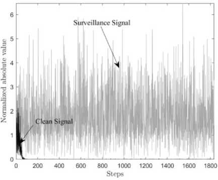
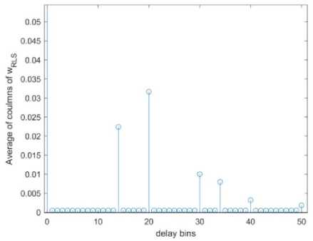
Fig.2. Computing clutters range and amplitude.

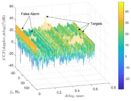
Fig.3. Target detection of RLS employing error-based clean signal.

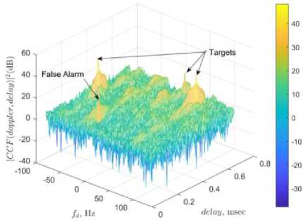
Fig.4. Target detection of RLS employing weight matrix-based clean signal.

Table 5. Error-based RLS compared to Weight matrix-based RLS.

RLS algorithm	Error-based	Weight matrix-based
CA	37.4450	54.4657
Complexity	1.3209e9	1.3235e9

The ambiguity functions are plotted for error-based and weight matrix-based LMS in Figs. 5 and 6. Employing the proposed weight matrix-based algorithm, CA is considerably improved (Table 8) and targets are detected (Fig. 6) in spite of some false detection in a few Doppler coordinates.

Fig.1. Clean signal after implementing RLS algorithm.

Table 6. Comparison of factual and evaluated clutters parameters in LMS.

Clutters	#1	#2	#3	#4	#5	#6
Factual Amplitude	22.36	7.07	2.23	1.25	15.83	5.61
Evaluated Amplitude	22.34	7.08	2.25	1.28	15.82	5.62
Evaluated Doppler	2.99	1.999	0.996	1.003	1.997	2.995

Table 7. Error-based LMS compared to Weight matrix-based LMS.

LMS algorithm	Error-based	Weight matrix-based
CA	32.4470	54.4563
Complexity	10.30e6	10.71e6

C. Simulation results of FBLMS scheme

The weight matrix *^ FBLMS is computed in this subsection. Initial filter iteration is chosen equal to Р =7 е 3. A larger initial filter repetition is required here in comparison to two previous methods, since convergence has a slower pattern. Clutter ranges are computed precisely similar to Fig .2, by plotting the average of weight matrix columns (14).

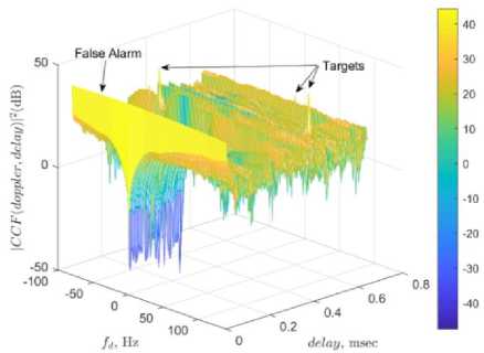
Fig.5. Target detection of LMS employing error-based clean signal.

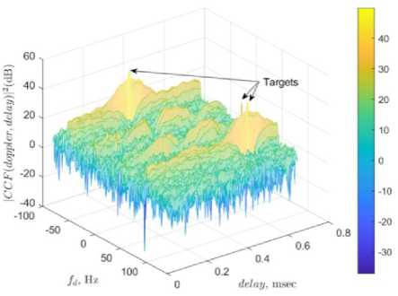
Fig.6. Target detection of LMS employing weight matrix-based clean signal.

A Comparison of factual and evaluated clutter parameters is provided in Table 8. Furthermore, CA and complexity are compared for error-based and weight matrix-based FBLMS in Table 9. The ambiguity functions are plotted for error-based and weight matrixbased FBLMS in Figs. 7 and 8. Compared to LMS, the weight vector is updated every М step in FBLMS. Therefore, the method is inappropriate for moving clutter cancellation (Fig.7). The false detection in Fig.7 is a result of relatively coarse approximation of Doppler and amplitude computed in Table 8. However, the much lower computational effort of FBLMS among all other methods is a supremacy. Tables 5, 7 and 9 prove that the clutter attenuation is much more powerful in case of weight matrix-based algorithm, while the computational effort is not increased much.

Table 8. Comparison of factual and evaluated clutters parameters in FBLMS.

Clutters	#1	#2	#3	#4	#5	#6
Factual Amplitude	22.31	7.05	2.23	1.25	15.79	5.60
Evaluated Amplitude	21.86	7.00	2.23	1.26	15.66	5.49
Evaluated Doppler	2.969	1.979	0.996	-0.995	-1.979	-2.968

Table 9. Error-based FBLMS compared to Weight matrix-based FBLMS.

FBLMS algorithm	Error-based	Weight matrix-based
CA	24.1838	49.1314
Complexity	3.6086e6	3.8612e6

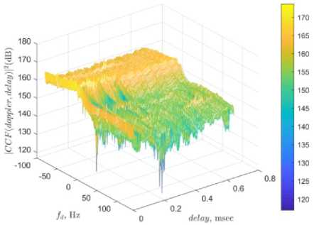
Fig.7. Target detection of FBLMS employing error-based clean signal.

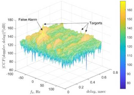
Fig.8. Target detection of FBLMS employing weight matrix-based clean signal.

D. Simulation results of ECA-B scheme

A very interesting application of the weight matrixbased approach is in ECA-B scheme. In this algorithm, signals are divided into N_b batches and 2 M„Ь + M_ab + M„ number of complex products is required in each batch, where N_b = N/ b and Mi is the dimension of column space of augmented matrix Hi In conventional ECA-B, the clean signal is computed in each computational batch, by minimizing the error in (7). Six Doppler defined in Table 1 along with the zero Doppler (which corresponds to direct signal) result in M_a = 7M. Also, number of data b in each batch is arbitrarily assumed equal to M to resemble a similar condition to FBLMS scheme. Note that, increasing M_a results in a high computational cost. Moreover, the pre-knowledge of clutters Doppler is an irrational assumption.

Next, the proposed method is examined to find the clutter properties from the weight-matrix, while augmentation of H is no longer required. Therefore, its column dimension is M. Clutters amplitude, delay and Doppler are evaluated from (14) and (15). Similar to Fig. 2, average of weight matrix columns reveal the exact ranges from (14). Table 10 compares the factual and evaluated Doppler and amplitudes computed from the weight matrix W ECA_B . Table llcompares the complexity of error-based and weight matrix-based schemes of ECA-B. The CCF plot for error-based ECA-B and Weight matrix-based ECA-B are shown in Figs. 9 and 10.

Although target detection is dropped down in weight matrix-based scheme, the complexity is considerably reduced. Tables 9 and 11 declare that the clutters evaluation precision of FBLMS and ECA-B algorithms (in weight matrix-based scheme) is less compared to other algorithms. The less computed CA is a result of the less precise clutter evaluation displayed in Tables 7 and 10.

Table 10. Comparison of factual and evaluated clutters parameters in ECA-B.

Clutters	#1	#2	#3	#4	#5	#6
Factual Amplitude	22.36	7.07	2.23	1.25	15.83	5.62
Evaluated Amplitude	21.23	7.08	2.24	1.26	15.81	5.58
Evaluated Doppler	3.0310	2.019	1.018	-1.017	-2.021	-3.032

Table 11. Error-based ECA-B compared to Weight matrix-based ECA-B.

ECA-B algorithm	Error-based	Weight matrix-based
CA	54.4254	49.1165
Complexity	7.4235e9	111.78e6

The reason is simply that the rows of weight matrices in both FBLMS and ECA-B are not updated in each step but the update is provided for each batch. Obviously, ECA-B could not detect targets similar to FBLMS in Fig. 7, if the H matrix was not augmented by considering all clutter Doppler shifts. Therefore, the moving clutter cancellation of batches algorithms like ECA-B and FBLMS (under the error-based scheme) is disproved.

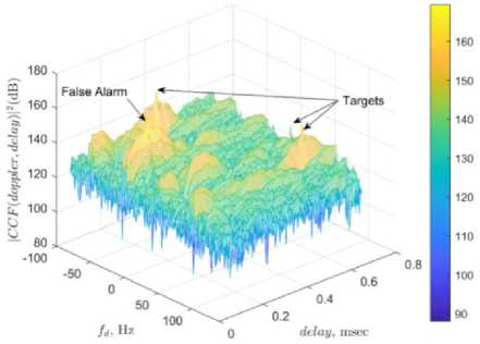
Fig.10. Target detection of ECA-B employing weight matrix-based clean signal.

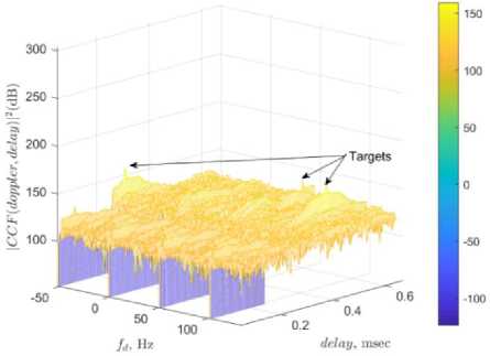
Fig.9. Target detection of ECA-B employing error-based clean signal.

A ppendix A the F blms A lgorithm

The row space of H matrix in (5) is divided into N _m batches. Each partition is called a row-batch. Vectors are denoted     by     underline.      The      weights

w(k) = [w ₀ ( k") ... w_M _!_ (k)] ^T are multiplied to each row of the k-th row-batch of H as follows:

У (kM)        = XML- ¹ w f ( k)S_ref [ kM-i ]

у(kM + M - 1) = XML-¹ W-(к)5_Г[ДкМ - i + M - 1]

Define   y(к) = [y(kM).. y(kM + M - 1)]T and

s (k) = [Sref\kM - M ]„.Sref[kM + M-1]]T,       A

Fourier transform algorithm is pursuit to compute y( k) with less computational effort. Denote the flipped vectors у and s by y _p and S p . If the FFT transform of S p is denoted by S f , then the i-th component of S f is denoted as S_Pl = Z 2M_o" ¹ 5_геДкМ + M - 1 - Z] e "² -^{й( 2M}) . Now, define

- ^{= FFr}[flB^(k) ]            (17)

L” ) Mx 1-1

by adding M zeros at the end of w(k). The components of y(k) are extracted by rewriting the product of Fourier transforms of SPi and — as follows:

- *Sp _t =

Z.?/ J Z 2 M: ¹ w^(fc)S _re/ [kM + M -1- I ] e " ^2j™s

= e "² ^^^^„(^S^^M + M - 1 - n]

+ — + e " ²^Z M^d w*(fc)S r_e/ [kM - n]

. ,2M-1

+e "^{2 ]т}Тм C _o + e ^jm 2 м C_M_ ₁

Looking at (16), the second line in (18) can be interpreted as:

e"2^я1^1у(kM + M - 1) + — + e"2j7ri^Ty(/cM)(19)

It is obvious then from (18) that y(k) is computed from:

[^] = I FFT {[FFT (^k) )]* x FFT(Sf)}(20)

where, x denotes element-wise product of vectors and C = [C _o ^ C _M" -J defines remaining coefficients in (18). Now, the convergence error is obtained from

Г e (kM)    1 Г    Ssu„[kM]1

e(к) = I         •         1 = 1           •           I - y(k)

[e(kM + M - 1)]   LS _SU rv [ kM + M - 1]J

The weight vector is updated in each batch step from и ( к + 1) = w(k) + 5w(k), where 5w(k) is evaluated by accumulating the product of e * (k) and each row (in the k-th row-batch of //matrix) as:

5w (k) = Z"o ^j e * (kM + i) *

(S _r gf [kM + i] ...  S _r gf [kM + i — M + 1]) ^   (22)

Let's rewrite 5w(Zc) = [5wo(/c)  ...  5 wM" 1(fc)]r as a columns vector, where:

5wj (k) = Z^o ^j e * (kM + i)S _ref [kM + i - j]   (23)

holds for j = 0, ...,M - 1. The M-length error vector e (k) is padded at the end with M zeros and a 2M-length FFT is computed as:

• - = ^{FFT [} 0)( xi ) ^] -

• Then, the i-th element of - and S = FFT(s(k)) are respectively defined as:

E_t = ZM^o ¹ e(kM + n)e "^{2 j} “ SM ,

S i = Z 2M_o" ¹ S_ref [kM - M + Z]e "^2j“ SM .

It is demonstrated next that a revision of the product of S i and E * guides one to compute И(_к). Let's write:

S- * =

ZSZ2Mo" 1 e*(kM + n)5re/[kM + M - 1 - I] e"2^ = e"2 j тТм Dq + e"2j“SM ZM^o1 e*(kM + n)Srgf[kM - M + n + 1] + .„ + e"2 j ^ZM-o1 e*( kM + n) Srgf[kM + n] +

„ . ,M+1                 „ . ,2M-1

e ^2jm 2м п_г + — + e ^{21 m} 2м d _M " ! .

The second line of above equation reveals the elements of Sw(/c) denoted in (23) as:

. , 1

e"2 jm2M<5wM " 1 (k) + — + e"2 j ^^„(fc)(24)

Define Sw f as the flapped vector 5и. Then 5и is computed from:

D₀ 6Wf (k) D

=

{[FFT( e(k) )]*xFFT(s)} I       \U)Mx 1 /)

The algorithm in Fig .11 elaborates in details, the required steps of implementing the complex-FBLMS method:

Eventually, the weight matrix IV_PBLMp is constructed similar to (12), by updating its rows in each batch step. In this algorithm an aggregate number of 6 FFT and IFFT which requires 2M I о g(MM ) multiplication each, and also other 16M multiplication is implemented in each batch. The convergence rate improvement algorithm which is applied in is also considered in above computation. Then, the whole complexity is evaluated by (12 (2 ) + 16 ) number of complex products.

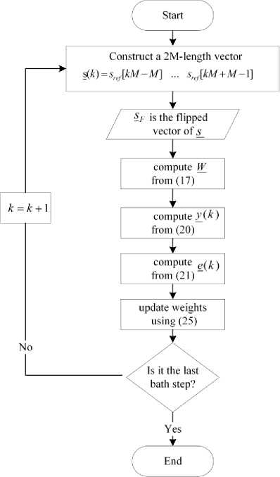
Fig.11. An algorithm to explain the complex FBLMS formalism.

• V. C onclusion

A weight matrix is extracted in iterative disturbance cancellation filters. It is then shown that this weight matrix can be employed effectively as a revealing source of clutters properties. A weight matrix-based scheme is innovated to progress the existing disturbance cancellation algorithms. The scheme upgrades the RLS, LMS, and FBLMS schemes in terms of clutter attenuation (CA), while the complexity is not much increased. Weight matrix-based LMS has the most acceptable results in preserving low computation along with high enough CA. Also, FBLMS formalism is revised to cover the case of complex input signals. Then, it is elaborated that FBLMS which is inadmissible for moving clutters cancellation, can remove the non-stationary clutters by employing the weight matrix-based scheme. Moreover, the method is applied for the ECA-B algorithm and compared to conventional ECA-B, the complexity is largely reduced. However, CA metric is slightly decreased. The weight matrix-based target detection scheme can be examined and compared for different filters in further investigations.