Wideband Direction of Arrival (DOA) Estimation: A Comparative Study of Wideband MUSIC Method, Joint Diagonalization Structure (JDS) Method and Beam-Space Genetic Algorithm (BGA)
 Estimation: A Comparative Study of Wideband MUSIC Method, Joint Diagonalization Structure (JDS) Method and Beam-Space Genetic Algorithm (BGA)")
Автор: Sandeep Santosh, O.P.Sahu
Журнал: International Journal of Information Technology and Computer Science(IJITCS) @ijitcs
Статья в выпуске: 9 Vol. 8, 2016 года.
Бесплатный доступ
In this paper, a comparative study of Wideband MUSIC method, Joint Diagonalization Structure (JDS) method and Beam-Space Genetic Algorithm (BGA) is presented with respect to resolution probability and Root mean square error (RMSE) evaluated in both low and high Signal-to-Noise ratio (SNR) regions. The simulation results show that BGA has higher resolution probability than the JDS method and Wideband MUSIC method in low SNR region while in the high SNR region, Wideband MUSIC has higher resolution probability followed by BGA and JDS method. RMSE is smallest for BGA as compared to JDS and Wideband MUSIC in low SNR region. In the high SNR region, Wideband MUSIC has smallest RMSE followed by BGA and JDS method.
Wideband Direction of Arrival estimation, Wideband MUSIC, Beam Space Genetic Algorithm (BGA), Joint Diagonalization Structure (JDS), Resolution Probability, Root Mean Square Error
Короткий адрес: https://sciup.org/15012544
IDR: 15012544
Текст научной статьи Wideband Direction of Arrival (DOA) Estimation: A Comparative Study of Wideband MUSIC Method, Joint Diagonalization Structure (JDS) Method and Beam-Space Genetic Algorithm (BGA)
Published Online September 2016 in MECS
In the field of navigation, oceanography, speech processing, communications, radar and sonar, we consider source localization using a sensor array [1],[2]. For estimation of Direction of Arrival (DOA) of narrowband sources, a number of high resolution algorithms like subspace fitting method [3], MUSIC [4], ESPIRIT [5] and Maximum-Likelihood method [6] are developed. For a narrowband signal, energy is located in a frequency band smaller than the central frequency. For applications like speech signal processing, seismic signal processing, passive sonars and high data rate communications, we consider the wideband signals. Wideband situations consider the ML methods in [7] and [8]. Coherent Signal Subspace method (CSSM) [9], [10], [11] is a high resolution Wideband Direction of Arrival estimation method. For determining the number of sources, the information theoretic criteria [12] are frequently used. The subspace based methods have a drawback that they consider that the number of sources are less than the number of sensors.
A high spatial resolution is a characteristic feature of Wideband MUSIC method [13]. For the Wideband MUSIC method, the number of sources are less than the number of sensors. Also, we must know in advance the number of sources, such that the noise space can be determined. The Joint Diagonalization Structure (JDS) [13] method is a one stage method i.e the DOAs are directly searched over the continuous location parameter space. In this method, it is not required to determine the number of sources before computing the spatial spectrum. Also, this JDS method considers that sensors number is not less than the number of sources. The beam-space Genetic algorithm is used for finding Direction of arrival of wideband signals. This is done by changing the array data to beam-space considering the frequency invariant beam forming matrix [14],[15].
In this paper, a comparative study of Wideband MUSIC method, Joint Diagonalization Structure (JDS) method and Beam-Space Genetic Algorithm (BGA) is presented with respect to resolution probability and Root mean square error (RMSE) evaluated in both low and high Signal-to-Noise ratio (SNR) regions. The simulation results show that BGA has higher resolution probability than the JDS method and Wideband MUSIC method in low SNR region while in the high SNR region, Wideband MUSIC has higher resolution probability followed by
BGA and JDS method. RMSE is smallest for BGA as compared to JDS and Wideband MUSIC in low SNR region. In the high SNR region, Wideband MUSIC has smallest RMSE followed by BGA and JDS method.
This paper has been organized as follows. Section 1 contains the introduction, Section 2 gives the Data model for wideband DOA estimation using JDS method and Wideband MUSIC method, Section 3 explains the use of Beam-Space Genetic Algorithm, Section 4 gives the Simulations, Section 5 contains the conclusion.
-
II. D ATA M ODEL FOR W IDEBAND DOA E STIMATION U SING JDS M ETHOD AND W IDEBAND MUSIC M ETHOD
N wideband sources encroach on M sensors arranged in a uniform linear array (ULA) having inter-sensor distance d as shown in Fig. 1.
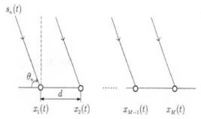
Fig.1. Uniform linear array of M sensors with interval d.
Consider the reference point as the first sensor. The signal of the nth source is denoted by sn (tc) and the continuous time index is represented by tc . The mth sensor receives the following signal [13], xm(tc)= 2N=1 ansn (tc-Tnm )+zm (tc), m=l,2,^,M (1)
The additive white Gaussian noise is denoted by zm(tc) , attenuation factor is denoted by an and propagation time - delay is represented by Tnm,
T nm =(m-1) d co^ (2)
The Direction of arrival of the nth source is 0< 9n < n and the propagation speed of the waveforms is represented by v.
Apply the short-time discrete time Fourier transform (ST-DTFT) on both sides of (1). Stack the ST-DTFT domain data of M sensors into a vector.
x (to,t) =[x1 (w,t) ,^., xM (tod)]T(3)
x (to, t) ^n ! sn (n,t)a(n, 9n) + z(to,t)
Where a(to, 9) is the array response vector in spatial-frequency domain and is defined as,
a(to, 9)= [i,e -jk“cos0
e —j(M—1)kwcos0 ] T
k = fs d/v k is a constant, d is the inter sensor spacing, fs = 1/Ts where Ts is sample period.
The matrix formulation of (3) is, x (to,t)= A(to)s(to ,t)+ z(to,t)
Where
s(n, t) |s,(n,t), ...,sN(to,t)]T
Where
z(to,t)= [zi(to,t), ™,Zm(to,t) ]T
s(to, t) and z(to, t) are the ST-DTFT data vectors of the source and noise respectively.
The M * N matrix,
A(to) = [a(to, 91 ),™,a(to, 9N)]
is the array manifold matrix in the spatial frequency domain.
The correlation matrix of the ST-DFT data vector x(to, t) is given as,
R x(to,t)=E[x(to ,t)x H (to, t)] (11)
Where E[.] represents the expectation and the superscript (.)H is conjugate transpose.
We define F(to) and G(to, 9) as follows,
F(to) = S K =1 R H (to,tk )R x (to,tk) (12)
G(to,9) = [R H (to^Oata,9),... ,R H (to,tK)a(to,9)
Where Rx (to, t) is given by (11) and a(to, 9) is given by (5).
All frequency components are integrated by the cost function of θ and is denoted by,
T-i minJ(9) = ^ (M - maxeig (GH(to, 9) Ft(m)G(m, 9))) n=i
Where F(to) and G(to, 9) are given by (12) and (13). The Moore-Penrose pseudo inverse is represented by the subscript (. ) ^ .
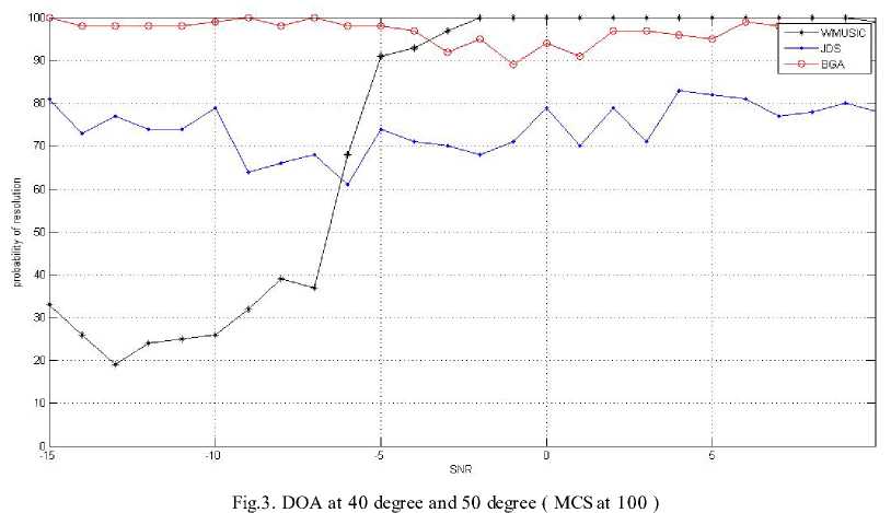
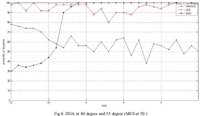
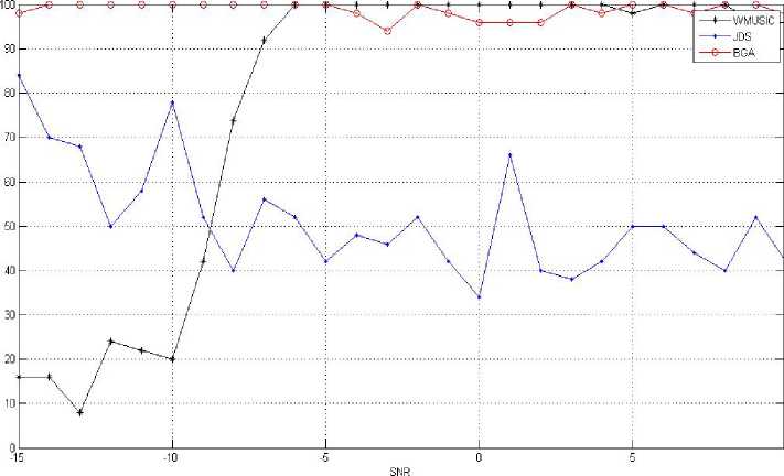
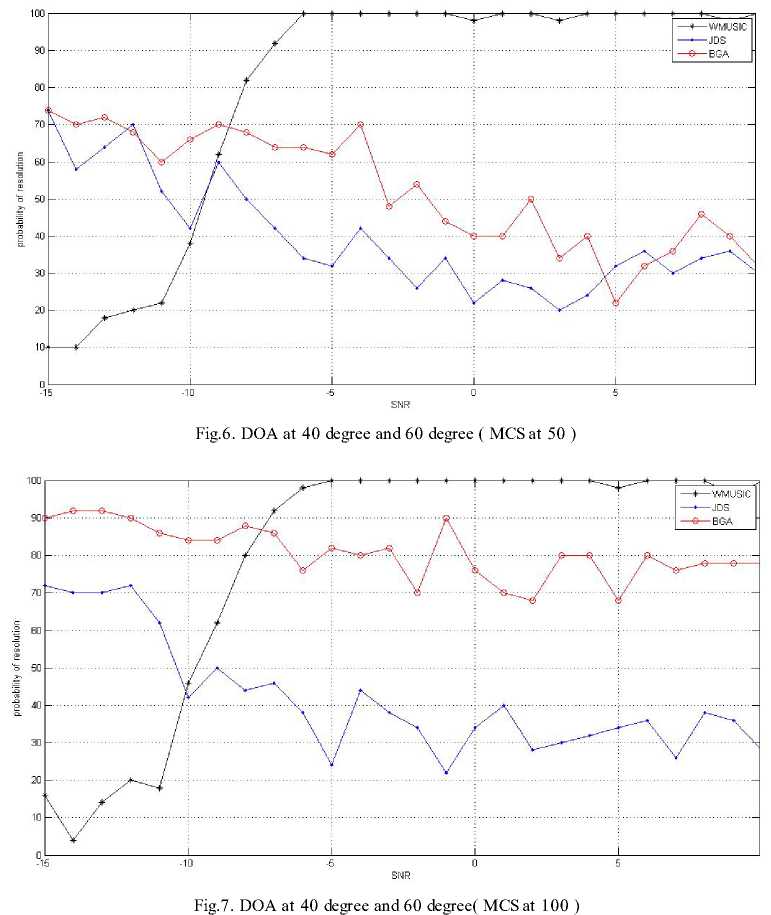
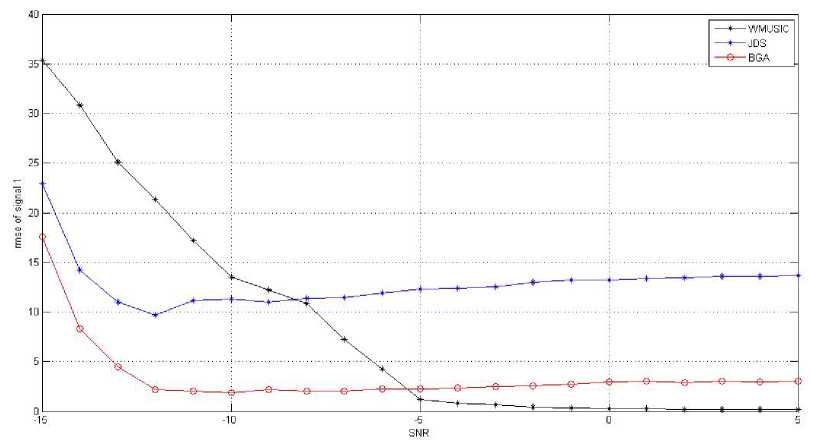
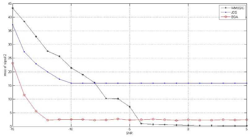
to = 2n (^) (1 Non stationary and wideband source is estimated by spatial spectrum represented by the following equation, P (0) =--------—-----1---------------- (15) m(— -1)-22_и max eig (GH(w,0)F^(w)G(ш,0)) 2 1 The maxima of P(0) can be searched which results in the detection and estimation of DOAs. By considering the sources and noise to be stationary, it results in Wideband MUSIC approach which is a special type of JDS method for K=1, where K is the short-time power spectrum matrices. The spatial spectrum of the JDS approach is simplified as, P(0) I K=i =---------------T-------------------------- M (T- 1) - Z^aHfe0)PRx(w)a(w, 0) PRx (to) = Rx(to) (RH(to)Rx(to))fR"(to) (17) PR[nrj(to) = Us(to)(UsH(to)Us(to))fU"(to) = Us(to)UsH(to) Us (to) represents signal subspace’s orthogonal basis. The concept of Us (to) is explained as below. Under the stationary assumption, Rx(to, t) is equal to R x (to). Rx(to) = A(to)Rs(to)AH (to)+ Rz(to) The eigen value decomposition (EVD) of Rx (to) is given by, Rx (to) = Us (to)A(to) Us H (to) Where, Atto = dia{A1 (to),A2 (to) ...,AM (to)} (21) is a diagonal matrix with, Ai(to) > A2 (to) > ••• > Am(to) > 0 being the nonnegative eigen values. The orthogonal matrix Us (to) is given as, Us (to) = [u1(to),u2(to),... ,uM (to)] (22) (22) contains M corresponding eigen vectors. Assume that number of sources N is known and N < M, we can make a basis of the noise subspace Uz (to) by the M-N eigenvectors corresponding to the last M-N eigen values as given below, Uz(to) = [uN+1 (to),uN+2(to), .,uM(to)] The space occupied by the noise-removed matrices Rxnr (to) has the projection matrix on it. P(0) Ik=i =--------т^-----1 (24) м(Т-1)-2Х2—1аН(ш,0)и5(ш)иН(ш)а (ш,0) The noise subspace is orthogonal to signal subspace, P R[nr] (to) = Us (to)UsH (to) = I - Uz (to) U" (to) P(0)lK=i T-i = 1/ ^ aH(to,0)Uz(to)UH(to)a(to, 0) = n=i PMUSIC(0) For the case of noise-removed matrices, a special case of JDS method can be taken to be the Wideband MUSIC method [13]. III. USE OF BEAM-SPACE GENETIC ALGORITHM The beam-space Genetic algorithm is used for finding Direction of arrival of wideband signals. This is done by changing the array data to beam-space considering the frequency invariant beam forming matrix [14]. Wideband Signal Model: We consider P wideband signals and M isotropic antenna elements for a linear array. The array output vector in frequency domain is obtained by considering that P wideband signals have similar bandwidth and similar SNR at various frequencies. Xj = A(fj, e)s(fj) + N(fj), j = 0,1,., J - 1 N(fj) = [Ni(fj)N2(fj)..NM(fj)]T J discrete frequencies compose the bandwidth. At frequency f , A(fj, 9)is the M*P array manifolds matrix. 9 = [90 91......9P-1]Tfor the ith source, 0, is the Direction of arrival. S (fj) represents the source vector for frequency f . N(fj) represents the noise vector for frequency f . Change the array output X(f) by the following equation with, Y(f) = B H(f, a)X(f) (31) where B(f, a) is given as w1 (f )e-v2”/'ri(“i) w2 (f )e-7'2’ry’T2(«i) wM (f )e-72,r^T«(ai) ... W1(f)e-72”/Ti(“L) ... w2(f)e-;2”/T2(“r) wM (f)e-72”^™(“r) is the beam forming matrix with constant beam width.Y(f) = [Y1 (f), Y2 (f), ., YL(f)]T is output of beam-space. Wi(f) is constant beam-width beam former’s weights (i=1,2,3, ,„,M) , тт(аг) is the corresponding time delay. Beam-space genetic algorithm (BGA): 1. With respect to the reference frequency f0 ,for every frequency in the frequency range, find the constant beam-width weight’s wi , i=1,2,…M. 2. For each discrete frequency, find the beam forming matrix. 3. Find beam-space output matrix at every frequency and get the output matrix Y(f0) at reference frequency by averaging each frequency together. 4. Find the DOA estimation by considering the conventional Genetic algorithm. IV. SIMULATIONS Consider twelve sensor ULA and sensor distance of 0.15 m and compute BGA through computer simulations. Take 50 and 100 Monte Carlo simulations (MCS) and 100 population and find the statistical performance. Two Gaussian white noise sources with similar bandwidth varying from 3 kHz to 7 kHz and same power are considered. The frequency of sampling is 14.05 kHz. 32 frequency bins are used [14]. Fig.2. DOA at 40 degree and 50 degree ( MCS at 50 ) Fig 2 shows the DOA at 40 degree and 50 degree and MCS at 50. The figure is a plot of SNR on x-axis v/s probability of resolution on y axis for WMUSIC, JDS and BGA method. For BGA method, the probability of resolution is highest and is about 100 for both low SNR and high SNR values. For JDS method, the probability of resolution decreases from 80 to 30 for low SNR values and it remains around 30 for high SNR values. Wideband MUSIC has smallest probability of resolution that increases from 20 to 40 at low SNR values and it shoots to around 100 at high SNR values. Fig 3 shows DOA at 40 degree and 50 degree and MCS at 100. The figure is a plot of SNR on x-axis v/s probability of resolution on y axis for WMUSIC, JDS and BGA method. For BGA method, the probability of resolution is highest around 100 for low SNR values and is around 95 for high SNR values. For JDS method, the probability of resolution decreases from 80 to 60 for low SNR values and it varies from 70 to 80 for high SNR values. For WMUSIC method, the probability of resolution varies from 30 to 40 at low SNR values and it shoots to around 100 at high SNR values. Fig 4 shows DOA at 40 degree and 55 degree and MCS at 50. The figure is a plot of SNR on x-axis v/s probability of resolution on y axis for WMUSIC, JDS and BGA method. For BGA method, the probability of resolution varies between 90 and 100 for low SNR values and probability of resolution varies between 80 and 100 for high SNR values. For JDS method, the probability of resolution decreases from 80 to 55 for low SNR values and it varies 50 and 60 for high SNR values. For WMUSIC, the probability of resolution increases from 30 to 60 at low SNR values and shoots to around 100 at high SNR values. Fig 5 shows DOA at 40 degree and 55 degree and MCS at 100. The figure is a plot of SNR on x-axis v/s probability of resolution on y axis for WMUSIC, JDS and BGA method. For BGA method, the probability of resolution is highest and is around 100 for both low and high SNR values. For JDS method, the probability of resolution decreases from 80 to 40 for low SNR values and is between 40 and 50 for high SNR values. For WMUSIC method, probability of resolution increases from 15 to 40 at low SNR values and it is around 100 at high SNR values. Fig 6 shows DOA at 40 degree and 60 degree and MCS at 50. The figure is a plot of SNR on x-axis v/s probability of resolution on y axis for WMUSIC, JDS and BGA method. For BGA method, the probability of resolution decreases from 75 to 65 for low SNR values and it decreases from 65 to 30 for high SNR values. For JDS method, the probability of resolution decreases from 75 to 55 for low SNR values and it falls from 55 to 30 for high SNR values. For WMUSIC method, the probability of resolution lies between 10 and 40 for low SNR values and it rises to around 100 for high SNR values. probability of resolution Fig.5. DOA at 40 degree and 55 degree ( MCS at 100 ) Fig 7 shows DOA at 40 degree and 60 degree and MCS at 100. The figure is a plot of SNR on x-axis v/s probability of resolution on y axis for WMUSIC, JDS and BGA method. For BGA method, the probability of resolution lies between 90 and 80 at low SNR values and it lies between 80 and 70 at high SNR values. For JDS method, the probability of resolution decreases from 70 to 40 at low SNR values and it lies between 40 and 30 at high SNR values. For WMUSIC method, the probability of resolution lies between 10 and 40 at low SNR values and it shoots to 100 at high SNR values. Fig.8. RMSE with signal 1 at 40 degree. Fig.9. RMSE with signal 2 at 50 degree. Fig 8 shows RMSE with signal 1 at 40 degree. The figure is a plot of SNR on x-axis v/s RMSE of signal 1 on y-axis. For BGA method, the RMSE is smallest and is around 17 and decreases to around 3 at low SNR values and at high SNR values it is around 4. For JDS method, the RMSE is around 23 and it decreases to 10 at low SNR values but the RMSE is around 13 at high SNR values. For WMUSIC method, the RMSE is highest around 35 and it decreases to 13 at low SNR values and it falls from 13 to 1 at high SNR values. Fig 9 shows RMSE with signal 2 at 50 degree. The figure is a plot of SNR on x-axis v/s RMSE of signal 2 on y-axis. For BGA method, the RMSE falls from 23 to 3 at low SNR values and it is around 3 at high SNR values. For JDS method, the RMSE falls from 37 to 16 at low SNR values and it is around 16 at high SNR values. For WMUSIC method, RMSE decreases fro 43 to 20 for low SNR values and it decreases from 20 to 1 at high SNR values. V. CONCLUSION The BGA has higher resolution probability than JDS method and Wideband MUSIC approach in the low SNR region. In the high SNR region, Wideband MUSIC has higher resolution probability followed by BGA and JDS method. The RMSE is smallest for BGA as compared to JDS and Wideband MUSIC in the low SNR region. In the high SNR region, Wideband MUSIC has smallest RMSE followed by BGA and JDS method.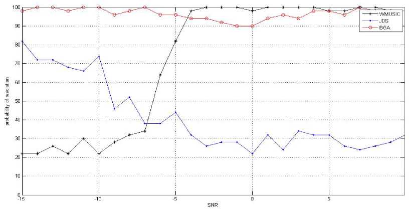
Список литературы Wideband Direction of Arrival (DOA) Estimation: A Comparative Study of Wideband MUSIC Method, Joint Diagonalization Structure (JDS) Method and Beam-Space Genetic Algorithm (BGA)
- H. Krim and M.Viberg, “Two decades of array signal processing research: The parametric approach”, IEEE Signal Processing Magazine, vol. 13, no.3, pp.67-94,July 1996.
- J.C. Chen, K. Yao & R.E. Hudson, “Source localization and beam forming”, IEEE Signal processing Magazine,vol.19,no.2,pp.30-39, March 2002.
- I.Ziskind & M.Wax, “Maximum Likelihood localization of multiple sources by alternating projection”, IEEE Transactions on Acoustics, Speech and Signal Processing, vol. 36, pp.1553-1560, October 1988.
- R.O. Schmidt, “Multiple emitter location and signal parameter estimation”, IEEE Transactions on Antennas propagation , vol. AP-34,no. 3, pp 276-280, March 1986.
- R.Roy & T. Kailath, “ESPIRIT- Estimation of signal parameters via rotational invariance techniques”, IEEE Transactions on Signal Processing, vol.37,no.7, pp 984-995, July 1989.
- M.Viberg & B.Ottersten, “Sensor array processing based on subspace fitting”, IEEE Transactions on Signal Processing, vol.39,no. 5, pp. 1110-1121, May 1991.
- Y.S.Yoon, L.M. Kaplan & J.H. McClellan, “TOPS: New DOA estimator for wideband signals, IEEE Transactions on Signal Processing, vol.54, no.6, pp.1977-1989,June 2006.
- M.A. Doron, A.J.Weiss & H.Messer, “Maximum Likelihood direction finding of wide-band sources”, IEEE Transactions on Signal Processing, vol.41, no.1, pp.411-414, Jan 1993.
- J.C.Chen, R.E. Hudson & K.Yao, “Maximum-likelihood source localization and unknown sensor location estimation for wideband signals in near field”, IEEE Transactions on Signal Processing, vol.50, no.8, pp.1843-1854, August 2002.
- H. Wang & M. Kaveh, “Coherent signal subspace processing for the detection and estimation of angles of arrival of multiple wideband sources”, IEEE Transactions on Acoustics, Speech and Signal Processing, vol. ASSP 33, pp. 823-831,August 1985.
- S.Valaee & P.Kabal, “Wideband array processing using a two sided correlation transformation”, IEEE Transactions on Signal processing, vol. 43, pp.160-172, January 1995.
- M.Wax & T.Kailath, “Detection of signals by information theoretic criteria”, IEEE Transactions on Acoustics, Speech and Signal Processing, vol. 33, no.3, pp. 387-392, April 1985.
- W.Zeng, & X.L.Li, “High resolution multiple wideband and non-stationary source localization with unknown number of sources”, IEEE Transactions on Signal Processing, vol. 58, no.6, pp.3125-3136, June 2010.
- J.Yong, J. Huang & J.Zhao, “Wideband Beam-space DOA estimation based on Genetic algorithm”,Third international conference on natural computation (ICNC 2007, IEEE 2007.
- Monika Agrawal and S. Prasad, "A Modified Likelihood Function Approach to DOA Estimation in the Presence of Unknown Spatially Correlated Gaussian Noise Using a Uniform Linear Array," IEEE Transactions on Signal Processing, vol. 48, pp. 2743-2749, Oct. 2000.
