Zero-Moment Point-Based Biped Robot with Different Walking Patterns

Published Online December 2014 in MECS

Since biped robots are desired to behave as humans do, they should have a certain level of intelligence [1]. In addition, a high level of adaptability should be provided to cope with external environments. As well as, in certain circumstances, optimal motion is selected to reduce energy consumption during walking [1]. There are numerous approaches to generate biped locomotion as detailed in [2-5]. Most researchers concentrate on control and walking patterns of the biped robot during the SSP due to its instability and the short time of the DSP (it is about 20% during one stride of the gait cycle). However, incorporating the DSP into gait cycle is necessary to generate smooth motion of the COG/hip trajectory (the hip position could be considered as approximation of the COG position), and to stop and change walking speed as desired [6-8]. On the other hand, analysis of the DSP could result in challenging problems concerning stable walking patterns and control; the biped robot behaves as over-actuated system with constrained motion [9, 10]. In effect, most mobile robots undergo difficulties concerning motion planning and control [11] To enforce the target biped to move, the analyst should generate stable trajectories for the COG and feet; the angular joint displacements and their first derivatives can be obtained using inverse kinematics. Therefore, the first part of this paper focuses on planning methods used for generation of COG trajectory especially during the DSP. Three methods are investigated and compared to understand differences, if exist, between these methods. Then, two walking patterns with four different cases are considered to understand the behavior of feet motion and the effect of impact on the biped configuration. Consequently, four different feet trajectories are encountered. Piecewise spline functions are used to approximate the feet trajectories during the SSP; whereas, foot rotation during the DSP is exactly arc.

Above all, stability of biped locomotion is needed to be evaluated because these analyses depend on approximate model represented by inverted pendulum which can result in deviations of ZMP trajectories. Therefore, the last part of this paper introduces solutions to the above. First, it proposes a thorough algorithm to tune walking parameters (COG height, distance traveled by the COG, and the times of the SSP and the DSP) and to satisfy specified kinematic and dynamic constraints. Second, it derives exact trigonometric relationships for feet trajectories during the DSP rather than the piecewise spline functions used in some works such as [12, 13].

This can avoid deviations in the velocity and acceleration of the feet at the transition instances of the walking cycle resulting in continuous dynamic response for the biped mechanism.

The structure of this paper is as follows. Section II presents different walking patterns for ZMP-based biped robot. Section III shows comparative study of generation of walking patterns during the complete gait cycle, especially for the DSP. Whereas, Section IV introduces a simple algorithm for generating stable biped walking compensating ZMP deviations. Section V presents simulation results and discussions. Section VI concludes.

• II.    Walking Pattern Generators

Due to complexity of the biped mechanisms, most researchers have simplified the gait cycle of the biped walking to understand the kinematics, biomechanics and control schemes of them. Studies have shown that there are four essential patterns used for generation of periodic biped walking; please see [2, 3] for more details. Fig. 1 illustrates the third patterns grading from simple to complex configurations.

• A.    Pattern 1

It consists of successive DSP and SSP without subphases, as shown in Fig. 1(a) [17]. The swing foot is always level to the ground during leaving and striking the ground. The biped mechanism that adopts this pattern may undergo under-actuation during the SSP if one considers the ankle joints as passive joints. In contrast, if the ankle joints are active (powered), the system will be fully actuated with allowable ankle torque to keep the ZMP within the contact area of the stance foot. However, the legs constitute over-actuated system during the DSP. Huang et. al. [12, 13] have stated that this type of pattern could result in unstable walking due to the sudden landing of the whole sole on the ground at the beginning of the DSP. This drawback can be overcome by pattern 2.

• B.    Pattern 2

This is analogous to the first pattern with exception that the swing leg will leave and land the ground with specified angle, as shown in Fig. 1 (b). This results in smooth transition of the striking foot from the heel to the whole sole at the beginning of the DSP. It has been noted that adding toe and heel joints to the feet concerning this walking pattern are necessary to realize stable toe-off and heel-off phases respectively. Missing these joints means line contact of the tips of the feet with the ground resulting in potential instability. Both the DSP and SSP could consist of one phase.

• C.    Pattern 3

It is a modified version of the walking pattern 2; it consists of one SSP and two sub-phases of the DSP as shown in Fig. 1 (c). In the first sub-phase the DSP (henceforth called DSP1), the front foot starts to rotate about the heel tip until it will be level to the ground. The rear foot, meanwhile, is in full contact with the ground.

Then the rear foot will rotate about the front edge in the second sub-phase of the DSP (henceforth called DSP2).

For other possible walking patterns, see [2].

• III.    A Comparative Study for Generation of Biped Walking Patterns

• A. COG (Hip) Trajectory

It is verified that designing a suitable hip trajectory can ensure stable dynamic motion for biped robots [12, 13]. We can classify two essential methods regarding this topic. The first one includes designing polynomial functions (or piecewise spline functions) for the hip trajectory during the complete gait cycle satisfying the constraint and continuity conditions [12-15]. This method selects the hip trajectory with largest stability margin represented by the ZMP stability margin.

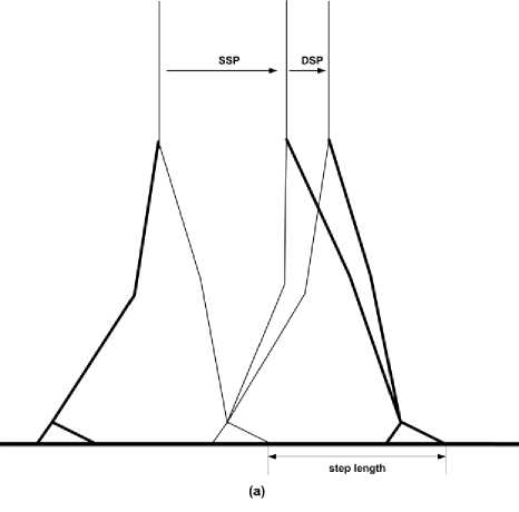
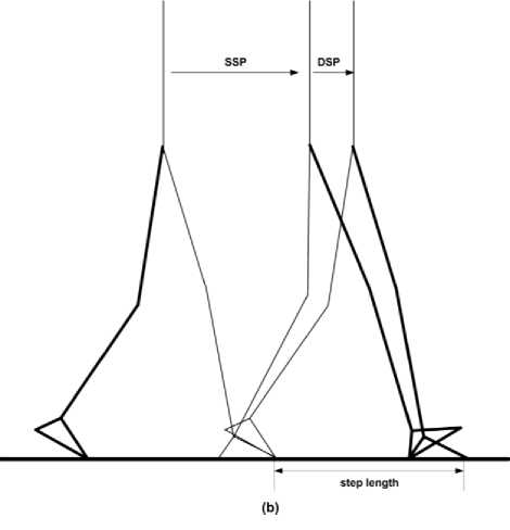
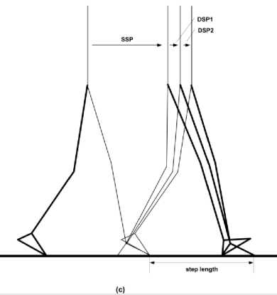
Fig. 1. Types of biped walking patterns. (a) Pattern 1, (b) Pattern 2, (c) Pattern 3.

In contrast, the second method suggests employing a simple dynamic model for the biped robot denoted by the linear inverted pendulum mode (LIPM) [6, 7, 16, 17]. Consequently, the notion of pendulum mode has been exploited for generation of stable hip motion. Designing walking pattern for biped mechanism without the DSP can lead to discontinuity of COG acceleration at switch (transition) instances as seen in Fig. 2; the DSP can mainly improve dynamic response at the expense of further computation. Below we will discuss three important methods used in literature for describing the motion of the COG trajectory during the two gait phases guaranteeing continuous transition between the phases. The following three methods have been used as walking generators for biped locomotion during complete gait cycle:

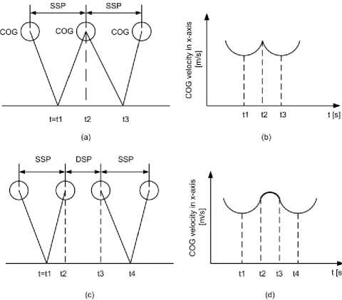
Fig. 2. (a) Biped walking patterns without incorporating the DSP, (b) COG velocity response without incorporating the DSP, (c) Biped walking patterns incorporating the DSP, (d) COG velocity response with incorporating the DSP

• •    Method 1: LIPM-based method [7]

In this method, both generation of walking patterns during the SSP and the DSP exploits the simplified model of inverted pendulum mode. Kudoh and Komura [7] have suggested a linear relationship between the ZMP and COG trajectories. In addition, they have considered the effect of the angular momentum at the COG of the biped robot; meanwhile, the classical linear inverted pendulum strategy assumes that no torques are applied at this point. Thus, we will modify the authors’ approach by assuming zero angular momentum and constant ZMP applied at the SSP for the sake of comparison with the next approach, as illustrated in Fig. 3. From the latter figure, the ratio of the ground reaction forces can be described as у ̈        - Рх

Лу⁼( ̈у+ д )=

where Л is the ground reaction force, с refers to the position of the COG (or the hip in this paper), р is the position of the ZMP trajectory, Н denotes height of the hip, and д is the gravitational acceleration. By assumption of no vertical motion, the relationship between the ZMP and COG trajectories can be described as

н..

=    -   ̈ s д s

The subscript S refers to the swing phase. Alternatively, (1) can be got from (2) by neglecting the angular momentum of the biped and assumption of ̈ У=0.

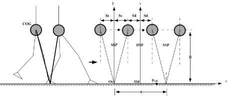
Fig. 3. Simplified modeling of biped robot based on method 1. Here ^s and Sд represent half of the distance spent by the COG during the SSP and the DSP respectively.

Because the ZMP is assumed fixed at the center of the stance foot in this work, the left hand side of (2) will be equal to zero. Consequently, the COG trajectory motion during SSP can be denoted by

Cx_s =       ( W_st )+ C_s2exp (- w_st )       (3)

where ^sl , C52 are constants which can be obtained from the boundary conditions, and

=

In similar manner, the relationship between ZMP and COG trajectories during the DSP can be expressed as

H ..

Vxd =    -   ̈

where c_Xd denotes the position of COG during DSP; ZMP trajectory can be assumed as

Рх^ =    /d-d(6)

where d^ refers to a constant that governs the walking parameters of the biped walking. Then, we can get the following equation

Cxd =       (wdt)+Cd2sin(wdt)

with wd =√9 (1/aa-1)/H(8)

To ensure continuous acceleration at the transition moment of the two phases, it is necessary that ( ̈=̈X)

at this moment. Thus, by substituting C =-Sд,= s^ in (2) and (5) we can obtain

Sd

Ss + §d = ad

If one select Sg and ^d as two independent variables, ^d. can be get from (9).

One of the important points lost in the above work is how to determine the suitable DSP time that corresponds with parameters S , Sd and Пд ; selection of the SSP and the DSP time is not arbitrary to ensure continuous dynamic response. This will be answered in the next method.

with p denotes a parameter that governs the biped walking, as we will see, and s is the step length. In addition

Sd^S

Cid =₂

As a result, we can obtain

O-d =1- P

and the position of the ZMP can be calculated as

^d =   / Cid =   /(1- P )         (14)

which is the same equation provided by [6]. By comparing (8) and (10), and substituting (13), we can get

H_d =(1- P ) H / P             (15)

which is the same equation obtained in [6]. Therefore, the two methods are equivalent and can give the same results.

Remark 1 . The correspondent value of the time of DSP ( Td ) that satisfies the constraint and continuity equation can be calculated as [6]

Td

= wd

(

^d ^хд (0) c*d ( Td)+ wdcXd(0) 2+

t ̇ _X_d (0) i ̇ _X_d ( ^ )

Wd

1 ^̇ Xd (0) ²

Wd

)

• •    Method 2: LIPM and LPM-based method [6]

In this method, an inverted pendulum is considered in the SSP and the same equations of the previous method we get; whereas, a LPM can be used for modeling the biped during the DSP as shown in Fig. 4. This method was suggested by Shibuya et al. [6] to relate the ZMP linearly to the COG trajectory. Interestingly, the same (5) is obtained during the DSP with motion frequency wd =√g/h;

with notations shown in Fig.4. Comparing the two mentioned methods (please see Fig.3 and Fig. 4), it can be noted that

Fig. 4. Simplified modeling of the biped based on Method 2

(1- p ) S

"d =

Remark 2 . From (13), we can notice the relationship between the parameter p and the parameter ^ad . As a result, a relationship between the parameter P and the time of DSP ( d ) should be considered to ensure a continuous motion, which is illustrated in (16).

Remark 3 . Following the work of [8], it is possible to consider the constraint relationship between the angle of the virtual pendulum ( бу ) and the coefficient of friction ( Ц ) as follows.

0≤ C0t6_v ≤ p               (17)

From Fig. 4, we can obtain

_{0≤   ≤} p               (18)

By selecting the values of s and H , a suitable value of p that satisfies (18) can be chosen. In brief, we can summarize the procedure for determining the COG hip trajectory of the biped during the one-step walking as follows:

• 1.    Determine the position of the COG of the biped robot.

• 2.    From (18), select the suitable values of p and s .

• 3.    From (16), determine the correspondent value of Td ; the step time and the swing time can be determined as Td ⁄0․2 and (0․8⁄0․2) Td respectively.

This depends on the mechanical design of the biped robot. Most researchers have tried to make the COG close to the hip position to simplify the calculations.

Using (3) and (7) and their 1st and 2nd derivatives, the motion of COG of the biped robot can be generated efficiently.

• • Method 3 [17]

This method suggests describing a suitable COG acceleration during the DSP satisfying continuous conditions at the transition instance. Vanderborght et. al. [17] suggested that two types of functions could be employed for this purpose. A linear acceleration at the DSP can be adopted to connect the previous SSP and the next one. However, a large computation can be arisen. Consequently, the authors suggested the same acceleration of the SSP can be used but with a negative sign. We will just display the equations required for the acceleration, velocity and the position of the hip trajectory during DSP. For details, we refer to the mentioned reference. We do not mention the case of the SSP because a simplified model of the inverted pendulum can be used during this phase.

схЛ t) = -cXs( t) = -(Cs iWi2exp(—Wi t) + cs 2 w/e xp (ws t))

Cxd t) = -(-Cs iWi exp(-ws t)

+ Cs 2 ws exp(ws t)) + c^CTJ + Wi (C12 — Ci1)

Cxd (t) = —(Ci iexp(—Wi t) + CS2 exp(wso)

+ (Cx_s(^Ti) + W i (C i2 - C i 1 )) t

+ C11 + C12 + CXs( Ti)

One of the disadvantages of this method is the discontinuity in the position of the COG. This can be solved by modifying the time of the double support phase to guarantee the continuity. This can coincide with the two previous methods in the selection of suitable T _d in order to guarantee continuous COG.

Remark 4 . All the mentioned methods above (1, 2 and 3) need compensation of the ZMP error due to approximation of the biped robot to pendulum model; the compensation technique will be explained in Section IV in details.

• B. Foot Trajectory

It is noticed that higher order trajectory may lead to oscillation and overshoot [18]. Therefore, it is desirable to use less order polynomials represented by piecewise spline functions to get the desirable dynamic performance for the biped robot. Huang et al. [12, 13] have employed piecewise cubic spline functions for interpolation of the foot trajectory. However, the authors have not assumed zero acceleration where the swing foot becomes flat on the ground (initial full contact). Therefore, Guan et al. [18] have suggested employing fourth order spline functions at the end segments with cubic spline functions for the intermediate segments to guarantee the zero constraint conditions at the end points. Depending on walking patterns 1 and 2, four cases are possible to be studied in order to see some differences of these walking patterns and the effect of impact from kinematics point view; please see Table 1 for more details.

• IV. A Simple Algorithm for Generating Stable Biped Walking Patterns

Despite miscellaneous walking pattern generation and stabilization approaches, it is difficult to find a thorough method that can tune the walking parameters to satisfy the kinematic and dynamic constraints: singularity condition at the knee joint, ZMP constraint, and unilateral contact constraints. Another problem that has been investigated in this section is generation of foot trajectory during DSP. References [12, 13, 19, 20] used piecewise spline functions to approximate the trajectory of the front and rear feet during DSP. It is known that during DSP the front foot rotates about the heel joint while the rear foot rotates about its front tip; therefore, their trajectories can be found easily by trigonometric relationships for arcs rather than approximate spline which can results in deviations in the velocity and acceleration of the feet especially at the transition instances. Therefore the following subsections propose a sufficient algorithm that solves the mentioned problems.

Remark 5 .

• •    The trajectory of the biped COG during the SSP and the DSP can be described using (3) and (7) respectively.

• •    Some of the drawbacks of walking pattern 2 have been described in [5]. Moreover, trajectory planning of walking patterns 2 and 3 could be similar; the difference is that motion of the front and rear feet during the walking pattern 2 are simultaneous, while their motion will be consecutive in walking pattern 3. In effect, the foot trajectory of the walking pattern 3 can be described as that of walking pattern 2 (case 3 in Table 1); the differences lie in timing the DSP ⁽ 1 1 = 0, t₂ ^—    = ^T d / ^2, t₄ — t₂ = T_s, t₅ — t₄ = T _d /

• 2) .

• A. Kinematic and Dynamic Constraints

• • Singularity constraint

There could be three reasons which may lead ZMP-based biped robot to walk with bent knees: (a) constraining the hip trajectory to move in constant height, (b) appearance of the difference of shank and thigh angles at the denominator in the inverse kinematics solution. (c) if the DSP is included in the trajectory planning, the constraint control (force control) of the biped could demand the same problem of (b) during solution. Applying the cosine’s law

c osQ = (222— D2 )/222           (36)

with Ω denotes the angle between the thigh link and the shank link, is the length of the shank link which is equal to the thigh one, and represents the distance between the ankle joint and the hip joint. To avoid singularity position for the knee joint, it is necessary to satisfy the following condition

— 1<(222 — D2)/222 < 1         (37)

Table 1. Description of different walking patterns for foot trajectory

Case No.	Description	Constraint conditions	The proposed piecewise spline functions
1	•    The foot is level to the ground without impact at instance of the ground-contact of the swing phase. •    The motion of one foot (the right foot) will be described; the other foot has the same motion.	•    x-axis: x ( (tj = —5 ,   xa(t2 ) = xobs ,  xa(t3 ) = 5 , xa (t i ) = Xa(t3) = 0,Xa(t1) = x a (t 3 ) = 0    (22) •    y-axis: y a(ti ) = 0, y a(t2 ) = y obs , у^ з ) = 0, ya(ti ) = ya(t3) = 0, ya(t i ) = y a (t 3 ) = 0     (23) where (xa, y a ) is the coordinate of the swing ankle, (xO b S,yO b S) is the coordinate of the obstacle position, t i = 0 , t2 = T d + T m and t3 = T d + T s , with T m represents the time required to cross the obstacle. У 2       _ Right foot Right foot | ________s__________ l Stance(left)       Right foot 1 foot Fig. 5. Foot trajectory for cases 1 and 2	f i (t) = ^^V(t —t i )^'   (t i 7 = 0 <    t < t 2 ) ^(t) =    ^P 2j (t — t 2 ) j   (t 2 j=0 <    t < t 3 ) (24) where Fi (.) represents x a or y a The   above   spline functions could briefly be called   4-4   piecewise spline functions.
2	The same walking pattern of case 1 but with impact at the landing.	•    x-axis:   x a (t i ) = -5 ,   x a (t 2 ) = xo6s ,   x a ( t 3 ) = 5, x a (t i ) = x a (t i ) = 0            (25) In effect, we have tried to connect the above constraint conditions using 3-3 piecewise spline functions, and 4th degree polynomial separately, but deformation of the trajectory would occur close to the instance of heel strike. Therefore, to get a feasible trajectory to be compared with other cases, we released the intermediate point at t = t2 for x- trajectory only; thus, we have four boundary conditions. •    y-axis: y a (t i ) = 0, y a (t2) = y obs , y a (t 3 ) = 0, y a( t i ) = y „ (t1) = 0     (26)	•    3 degree polynomial for x a trajectory. •    3-3 piecewise spline functions    for    y a trajectory.
3	•    The foot will swing and strike the ground with some specific angles. •    In this walking pattern, the rear and front foot of the biped during the DSP will move together; therefore, there is no sub-phases for the DSP (just one DS phase). •    The foot strikes the ground without impact. У V сл^ Л1           ; Right foot             g         iStaneofleft)        5 Right foot H foot Fig. 6. Foot trajectory for cases 3 and 4	•    The right foot during t i < t < t 2 (The foot will be in the rear position, see Fig. 6.) x a = —5 + l a cos(q 7 ), with nomenclatures shown in Fig. 6 (27) y a = l a Sin ( Q 7 )     (28) •    Swing foot trajectory , t2< t < t4 , (T = t4 — t2), (T D = t2 — ti) x-axis:  x a ( t2) = —5 + l a cosf^^)) , xafc) = xo6s , x a( t 4 ) = 5 — l a — l b + l b CoS^M — Л) xa(t2 ) = —la sint^Cti) q7(t2                           ). x a( t 4 ) = —l b sin ( q 7( t 4 ) — О q 7( t 4 )     ,      xa(t2) = — l a (sin(q 7( t 2 )) q 7( t 2 ) + CoS^y^)) q 7( t 2)2 ), x a( t 4 ) = —l b (sin ( q 7( t 4 ) — О q 7( t 4 ) + Cos(q7(t4) — я) q 7( t 4)2 )         (29) y-axis: y a (t2) = l a Sin(q i( t 2 )) , y afc ) = yo b s , ya(t4) = l b Sin ( q 7( t 4 ) — О y a (t 2 ) = l a COS ( q 7 (t 2 )) q 7 (t 2 ) , ya(t4) = l b cos(q y (t4) — я) q 7( t 4 ) ya(t2 ) = la(cos( q 7(t2 )) q7(t2 ) — sint^Cti) q7(t2)2) y a( t 4 ) = l b (cos ( q 7( t 4 ) — л) q 7( t 4 ) — Sin ( q 7( t 4 ) — ^)q 7 (t 4 ) 2 )   (30) •    The right foot during /4 < t < t 5 (The foot will be in the front position) x a = 5 —l a —l b + l b Cos ( q 7 — Я)    (31) y a = l b Sin ( q 7 — ^),    (32) •    Trajectory of foot angle Foot angle during the time  t i < t < t 4 :  q 7 (t i ) = n, q 7( t 2 ) = qP.q 7( t 4 ) = q h   ,   q 7( t i ) = q 7( t 4 ) = 0  , q 7( t i ) = q 7( t 4 ) = 0     (33) Foot angle during the time t4< t < t5 :  q7(t4) = q h , q 7( t 4 ‘ ) = q,q 7( t3) = n   ,   q 7( t 4 ) = q 7( t s ) = 0   , q7(t4 ) = q7(tS ) = 0     (34)	•    The front and rear feet will move as  arcs therefore, there is no need   for  proposed spline functions. •    The swing foot will move as 4-4 piecewise spline functions. •    The foot angle will move as 4-4 piecewise spline  functions  for both periods (t i < t < t4,t45)
4	The same walking pattern as case 3 but with impact at heel strike.	The derivation of x, y foot trajectory during the SSP and the DSP are exactly the same as that of the latter case; see (27) to (34). The imposed constraint conditions for the foot angle are: q 7( t i ) = n, q 7( t 2 ) = q p , q 7( t 4 ) = q h , q 7( t3) = n, q 7( t i ) = q 7( t5 ) = 0, q 7( t i ) = q 7( t s ) = 0 (35)	4-3-4 piecewise spline functions for the foot angle.

• Unilateral contact constraints

During SSP

| Лс|-Ц| лу|<0

(Non-slipping condition)

Лу>0

(Compressive normal force)

• •    . During DSP

| Л_х|- ц | Лу|<0   (Left foot: non-slipping condition)

Лу>0 (Left foot: compressive normal force)

| Л'_х|- ц | Л'у|<0   (Right: non-slipping condition)

Л'у>0

(Right: compressive normal force)

with л7 refers to one component of the ground reaction force at the right foot.

Remark 6. Since the biped robot does not have a unique solution during the DSP, we assume a linear transition function for the ground reaction forces of the front foot (right foot) as follows [5]

л=( - * Ш-сод ( ̈ сод+[0,д]) (41)

where ̈ =[ ̈ х ̈_{] ,} т is the mass of the center of gravity and ̈ сод represents the acceleration of the biped COG. Whereas the rear foot (left foot) has the following ground reaction forces:

Л' =      ( ̈ сод+[0,д])-л           (42)

Remark 7 . Since the biped robot does not have a unique solution during the DSP, we assume a linear transition function for the ground reaction forces of the front foot (right foot). For details, see [5, 10].

• •    Zero-moment point constraint

-

-к≤Р    ≤S   for DSP with

^∑ iUmi ( ̈ yi+S¹ ) ^cxi ^∑ i^l^mi ^{̈      ∑}E=i и ̈

^^real =               _∑ l^i^mi ( ̈ yi"*"3 )

where ТП[ is the mass of link (i), H is the number of links, Ц is the moment of inertia about COG of link (i), and ̈ i denotes the angular acceleration of link (i).

• B.    The Proposed Algorithm

To get feasible biped motion, the aforementioned kinematic and dynamic constraints should be satisfied. The proposed compensation algorithm can be described as shown in Fig. 7.

• V. Simulation Results and Discussions

The results can be divided into three categories as follows:

• A.    Comparison between Methods 1, 2 and 3

Following the procedure described in Section III for generation of COG trajectory, the desired (walking) parameters have been used are: (Л = 0․5, = 0․7561 (cases 1,2), p = 0․7575 (cases 3, 4), = 0․5 [ s ], Д = 0․125 [ s ].

It is noticed that there is clear relationship between the walking parameter p and Тд as expressed in (16). In effect, Methods 1 and 2 have exactly the same results; therefore, we confined our comparison between Methods 2 and 3. It is noted that the COG motion is continuous regarding position, velocity and acceleration, as shown in Fig. 8. The two methods give similar motion. However, Method 2 is more systematic in dealing with the parameters of the biped walking and guaranteeing the constraint and continuity conditions.

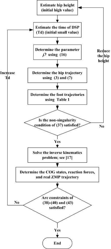
Fig. 7. Flow chart of the proposed algorithm for ZMP compensation

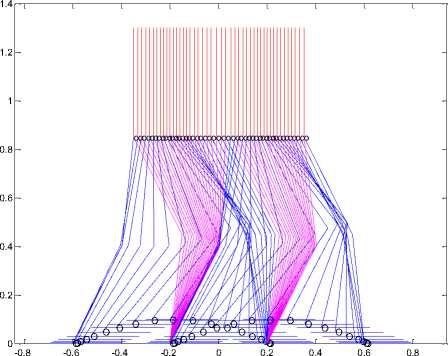
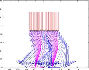
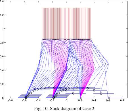
From Fig. 8, it is clear that the SSP encounters deceleration and acceleration sub-phases sequentially. This can be explained according to (2) where deceleration of the biped robot can occur until the middle of SSP because the COG position is behind the front stance foot. The next acceleration sub-phase can result from the progression of the COG in front of the stance foot. Another issue that can be noticed is that the motion of the hip link is close in the middle of SSP, as shown in Fig. 9 to Fig. 12.

• B.    Gait Patterns Based on Foot Trajectory

In this study, four cases of foot trajectory with different boundary conditions were compared as detailed in Table 1. The characteristics (advantages and disadvantages) of these cases are detailed in Table 2.

Table 2. The characteristics of foot trajectory according to the four simulated cases

Case No	Characteristics
1	•    The foot is level to the ground. •    The maximum hip height is 85 [mm]; increasing this value could result in singularity at knee joint. •    Due to zero velocity and acceleration at end conditions, the swing foot moves very slowly at these ends; this can lead more energy consumption especially at heel strike [17]. •    Due to the latter point, rather messing configuration of swing leg at the end of swing phase; see Fig.9.
2	•    The foot is also level to the ground. •    The maximum hip height is 85 [mm]; increasing this value could result in singularity at knee joint. •    There is some change in behavior of foot motion at the end of the swing phase due to free condition (striking the ground with some velocity) at this end. This may explain the uniform configuration of the swing leg at end of this phase, see Fig. 10. •    It is difficult to add intermediate point for foot trajectory in x-axis due to the free condition mentioned previously, see Table 1.
3	•    The foot takes off and strikes the ground with specified angles; see Fig. 11 . •    Although the biped robot strikes the ground without impact, its configuration can be improved by modifying landing angle as shown in Fig. 11 (a) and (b). •    The foot moves very slowly at the beginning and end of the swing phase due to its zero end conditions.
4	The foot trajectory has the same characteristics as that of case 3 but with some free motion at heel strike due to free impact at this instance; see Fig. 12.

• C.    Compensation of ZMP Deviations Using Algorithm of Fig. 7

All above analyses have been performed without checking whether the ZMP trajectory is still inside the support polygon or not. In this study, we concentrated on walking pattern 2 and 3. In general, the results can be summarized as follows:

• •    Walking pattern 3 before and after compensation.

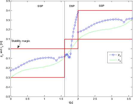
We selected initial parameters for our biped model (Н = 0.88m, а = 0.7557, T_d = 0.125 [s], T _s = 0.5 [s]) . In effect, these parameters have been selected according to previous work which deals with suboptimal trajectory planning of the same robot model. The proposed hip height of the biped can violate the singularity condition. Therefore, unreasonable solution can be obtained due to appearance of imaginary numbers. Our suggested algorithm tunes the mentioned parameters to give stable trajectory for the COG of biped model. Table 3 shows the walking parameters before and after compensation while Fig. 13 and Fig. 14 show COG and ZMP trajectories before and after tuning respectively.

• •    Walking pattern 2 vs. walking pattern 3.

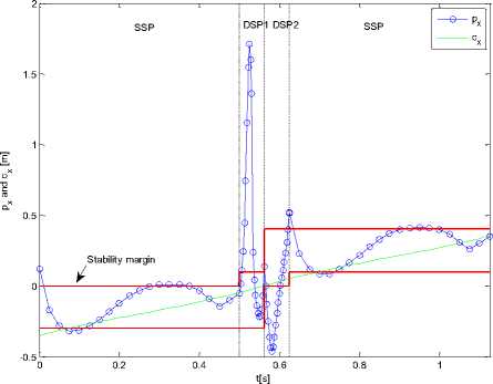
From Fig. 15, it could be noted that the ZMP is out of its stability margin at the beginning of the DSP due to rotation of the rear foot instantaneously at the DSP. This instability can be avoided in walking pattern 3 which can guarantee smooth transition or ZMP trajectory and foot rotation. In effect, keeping stance foot fixed at beginning of DSP is necessary to get stable motion.

Table 3. Tuning of walking parameters

	Walking parameters
Before compensation	Н = 0.88m,p = 0.5757, T d = 0.125 [s],Ts = 0.5 [s]
After compensation	Н = 0.86m,p = 0.6203, T d = 0.3 [s],Ts = 1.2 [s]

• VI. Conclusions

• •    In this paper, we have attempted to focus on the smooth transition from the SSP to the DSP and vice versa. Three methods have been compared for this purpose. The first two methods have exploited the notion of pendulum mode with different strategies. However, it is found that the two mentioned methods can give the same motion of center of gravity for the biped. Whereas, Method 3 has suggested to use a suitable acceleration during the double support phase (DSP) for a smooth transition. Although the Method 3 can give close results as in the former methods, the latter are more systematic in dealing with the walking parameters of the biped robot. The second issue we focus on is the different patterns of the foot trajectory especially during the DSP. The characteristics of foot rotation can improve the stability performance generating uniform configuration.

• •    The last part  of this  paper  concentrates on

compensating the ZMP deviations due to approximate model of LPM. Successful results can be got with walking pattern 3.

• All above methods are offline applied because it uses much iteration to get the feasible motion for the target biped. The online modified version should be tested and selected carefully as discussed in detail in chapter 3.

t[s]

(a) with contact angle of 120.

Fig. 8.The position, velocity and acceleration of COG (hip) (Method 2 ----; whereas Method 3___). As noted, the two methods have the same results.

(b) with contact angle of 300.

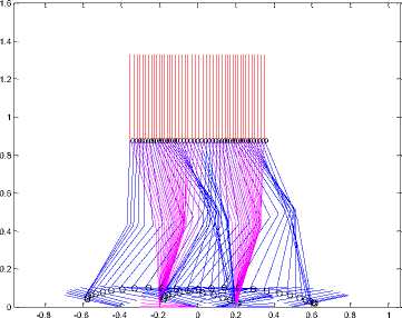
Fig. 11. Stick diagram for case 3

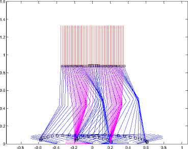
(a) Stick diagram of case 4 with contact angle of 120.

Fig. 9. Stick diagram of case 1

(b) Stick diagram of case 4 with contact angle of 30°.

Fig.12. Stick diagram for case 4

g. .                                                p                    g pattern 3)

• [2]    Hayder F. N. Al-Shuka, F. Allmendinger, B. Corves, and W.-H. Zhu,” Modeling, stability and walking pattern genartors of biped robots: a review,” Robotica , FirstView Article, pp. 1-28, 2013.

• [3]    Hayder F. N. Al-Shuka and B. Corves,” On the walking pattern generation of biped robot,” Journal of Automation and Control (JOACE) , vol. 1, no. 2, pp.149-155, 2013.

• [4]    Hayder F. N. Al-Shuka, B. Corves and W.-H. Zhu,” On the dynamic optimization of biped robot,”. Lecture Notes on software Engineering , vol. 1, no. 3, pp. 237-243, 2013.

• [5]    Hayder F. N. Al-Shuka, B. Corves, B. Vanderborght, and W.-H. Zhu,“ Finite difference-based suboptimal trajectory planning of biped robot with continuous dynamic response,” International Journal of Modeling and Optimization , vol. 3, no. 4, pp. 337-343, 2013.

• [6]    M. Shibuya, T. Suzuki, and K. Ohnishi,” Trajectory planning of biped robot using linear pendulum mode for double support phase,” Proc. IECON 2006-32nd Annual Conf. IEEE Industrial Electronics, pp. 4049-4099, Paris, 2006.

  

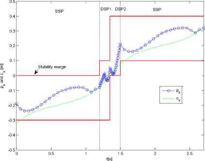
  Fig. 14. ZMP and COG trajectories after compensation (walking pattern

  
  

• [7]    S. Kudoh, and T. Komura,” C² continuous gait-pattern generation for biped robots,” IEEE/RSJ Intelligent Robots and Systems, vol. 2, pp. 1135-1140. Las Vegas, Nevada, 2003.

• [8]    C. Zhu and A. Kawamura, “Walking principle analysis for biped robot with ZMP concept, friction constraint, and inverted pendulum mode,” In Proc. 2003 IEEE/RSJ Intl. Intelligent Robotics and systems , vol.1, pp. 364-369 2003.

• [9]    Hayder F. N. Al-Shuka, B. Corves, Wen-Hong Zhu, and B. Vanderborght,” Multi-level control of zero-moment point (ZMP)-based humanoid biped robots: a review,” Robotica (accepted).

• [10]    Hayder F. N. Al-Shuka, B. Corves, and Wen-Hong Zhu,” Dynamic modeling of biped robot using Lagrangian and recursive Newton-Euler formulations,” International Journal of Computer Applications (IJCA), in press.

• [11]    V. Aenugu, P.-Y. Woo,” Mobile robot path planning with randomly moving obstacle and goals,” International Journal of Intelligent Systems and Applications (IJISA), Mecs , vol. 4, no. 2, pp. 1-15, 2012.

  

  g. .     a        a eco es a e co pe sao wa g pae

  
  

• [12]    Q. Huang, S. Kajita, N. Koyachi; K. Kaneko,“ A high stability, smooth walking pattern for a biped robot,” IEEE International conference on Robotics and Automation, vol. 1, Detroit, MI, pp.65-71, May 1999.

• [13]    Q. Huang; K. Yokoi, S. Kajita, K. Kaneko, H. Arai, N. Koyachi, K. Tanie,” Planning walking patterns for a biped robot,” IEEE Transactions on Robotics and Automation , vol. 17, no. 3, pp. 280 – 289, 2001.

• [14]    X. Mu, Q. Wu,” Synthesis of a complete sagittal cycle for a five-link biped robot,” Robotica: vol. 21, pp. 581-587, 2003.

• [15]    Z. Tang, C. Zhou, Z. Sun,” Trajectory planning for smooth transition for a biped robot,” IEEE International conference on Robotics and Automations, vol. 2, pp. 2455-2460, 2003.

• [16]    S. Kajita, S. and K. Tani,” Experimental study of biped dynamic walking,” IEEE, Control Systems, vol. 16, no. 1, pp. 13-19, 1996.

  References

  
  

• [17]    B. Vanderborght, R. V. Ham, B. Verrelst, M. V. Damme, D. Lefeber,“ Overview of the Lucy project: Dynamic stabilization of a biped powered by pneumatic artificial muscles,” Advanced Robotics , vol. 22, no. 10, pp. 10271051, 2008.

  [1] M. Vukobratovic, and J. Stepanenko,” On the stability of anthropomorphic systems,” Mathematical Biosciences , vol.15, no.1-2, pp.1-73, 1972.

  
  

• [18]    Y. Guan, K. Yokoi, O. Stasse, A. Kheddar,” On robotic trajectory planning using polynomial interpolations,” In Proc. IEEE Conf. Robotics and Biomimetics, pp. 111-116, 2005.

• [19]    L. Wang, Z. Yu, F. He, Y. Jiao,” Research on biped robot gait in double-support phase,” IEEE International Conference on Mechatronics and Automation, pp. 15531558, 2007.

• [20]    C. -L. Shih,” Gait synthesis for a biped robot,” Robotica : vol. 15, pp.599-607, 1997.