Звездные структуры в f(R)-гравитации в пространстве–времени Финча–Скеа

In 1913, the collaboration between Einstein and Marcel Grossmann laid the foundation for the general theory of relativity (GR) [1]. Despite its remarkable success in explaining cosmic evolution and accounting for dark energy (DE) and dark matter (DM), GR faces some challenges, like regarding the universe’s accelerated expansion [2, 3]. Observational evidence from Type Ia supernovae and the cosmic microwave background indicates that our universe is expanding at an accelerating rate [4], a phenomenon not fully captured by classical GR. This has motivated the exploration of modified theories of gravity, especially f (R) gravity, introduced by Starobinsky in the context of inflation [5]. In this extension, the Ricci scalar R in the Einstein-Hilbert action is replaced by a general function f (R) , which may include higher-order curvature terms such as R 2 . These modifications inherently alter the geometric side of Einstein’s field equations, allowing the geometric sector to mimic the effects of DE and DM [6]. modified theories of gravity, including f (R) , f (G) , f(G,T ) , and f (G,T 2 ) (with G being the Gauss–Bonnet term and T the trace of the energy–momentum tensor), have attracted significant interest in recent years [7–14]. These approaches provide a geometric alternative to explaining large-scale cosmic behavior without introducing exotic matter components. At stellar scales, anisotropy in pressure becomes relevant at high densities [15]. Recent studies highlight the substantial impact of pressure anisotropy on compact object configurations and their stability [16–21]. In anisotropic models, the mass–radius ratio ² _R ^M can approach unity, though isotropic models remain constrained by the Buchdahl limit ² _R ^M <   ⁸ ₉ [22]. Yazadjiev [23] introduced electric charge in solving the Einstein–Maxwell field equations to study highly magnetized systems like magnetars, showing how magnetic fields induce anisotropy. Strong magnetic effects have also been studied by Astashenok et al. [24] using f (R) gravity, revealing that quadratic Gauss-Bonnet terms can support massive neutron stars with high strangeness content. Gravitational wave detections from compact binary coalescence have recently identified compact objects with masses between 2.50 M q and 2.67 M q [25], challenging the conventional neutron star mass limits. These findings motivate further investigation of modified theories of gravity in describing extreme stellar structures. Additional studies explore how modifications to gravity affect the mass thresholds and stability of compact stars [26–31]. While GR provides a robust framework, it struggles to explain late-time acceleration without introducing a DE component [9, 11, 32–34]. Alternatives such as Modified Newtonian Dynamics (MOND) were proposed by Milgrom [35–40] to explain galactic rotation curves without invoking DM. MOND modifies Newton’s laws rather than Einstein’s, offering partial success on galactic scales but struggling with cosmological consistency. Scalar–tensor theories, such as those proposed by Dicke, incorporate scalar fields into gravity, modifying matter dynamics and potentially explaining the universe’s accelerated expansion [41–43]. While promising, these models face challenges including fine-tuning and equivalence principle violations [44–48]. Other approaches, like scalar–vector–tensor gravity, allow variations in ω , µ , and G , and provide potential explanations for structure formation and cosmic microwave background features, though they too are sensitive to parameter choices and observational constraints.

This study adopts a methodology tailored to the Finch–Skea geometric background to explore static, anisotropic fluid distributions in f (R) gravity. In the following section, we formulate the field equations for static, spherically symmetric spacetimes incorporating curvature corrections. Section 3 presents exact solutions and analyzes their physical acceptability. The concluding section summarizes the key results and insights derived from the analysis.

1.    Field Equations and Matching Conditions for Anisotropic Stars in f (R) Gravity

The f (R) theory of gravity is a natural generalization of Einstein’s General Relativity (GR), in which the Ricci scalar R in the Einstein-Hilbert action is replaced by a general function f (R) . The action for this modified theory is given by [9, 40, 49]

I = j V-g [f (R) + L m ] d ⁴ x,                                (1)

where g is the determinant of the metric tensor g^ , f (R) is a differentiable function of the Ricci scalar R , and L m represents the matter Lagrangian density. The volume element of the spacetime manifold is d ⁴ x .

Varying the action with respect to the metric tensor g µν leads to the modified field equations [50,51]:

R r R ^v - 2 g ^v f (R) + (g^ □ - VV ) f R = T^,                   (2)

where f R = dfR , □ = V ^м V _M is the d’Alembertian operator, and T^ is the energy-momentum tensor. For an anisotropic fluid distribution in a static spherically symmetric spacetime, the energy–momentum tensor is taken as [15, 16]

T Mv    ^{(p + p} r ^)U M U v + ^(p t ^p r ^)V M ^V v p t g Mv ,                           ⁽³⁾

where ρ is the energy density, p _r is the radial pressure, p _t is the tangential pressure, U ^µ is the four-velocity of the fluid satisfying U ^M U _M = 1 , and V ^м is a spacelike vector orthogonal to U ^м such that V ^m V m = - 1 .

These formulations extend the Einstein field equations and allow for richer gravitational dynamics, particularly useful in modeling compact stellar ob jects and addressing cosmological phenomena such as dark energy and late-time cosmic acceleration.

For a static spherically symmetric configuration, the general form of the line element is given by ds2 = ea^dt2 - eb^dr2 - r2(dO2 + sin2 Odf2),                         (4)

where e ^a(r) and e ^b(r) denote the temporal and radial metric potentials, respectively. In this study, we adopt the Finch–Skea metric [52], defined as:

e ^a(r) = ^ A + 1 b V C^ ,  e br = 1 + Cr ² ,                     (5)

where A , B , and C are constants determined through boundary conditions by matching with the Schwarzschild exterior at the stellar surface.

Solving the modified field equations of f (R) gravity, we obtain the following expressions for energy density, radial pressure, and tangential pressure:

- b

P = 2r 2 \f R ^Rb^b' + r ^{2 b}'f R + fe^br² + f R ^Rr²e^b - ^2г2& - 4rf R + 2f R e ^b - 2 Jr) ,         ⁽⁶⁾

- b

P r = - 2T 2 [f R rao! + r ² a'f R + 4rf R - 2 J r , e^b + 2 Jr, - fR.Rr²e^b + fr ² e^b) ,             ⁽⁷⁾

e - b

P t = ^T [f R Rra" + 2ra ' f'_R - f R ra'b' + f _R r(a')² - 2rb ' fR + 2J r o ! - 2R r b ' - 2rf R Re ^b + 2rfe ^b + 4f R + 4rf R ) .

The Ricci scalar R for this geometry is given by:

e ^{- b}

R =     (4 + r ² a ’² - 4e ^b + 2r ² a " - 4rb' + ra ' (4 - rb ' )) .

2 r ²

These expressions describe the internal structure of an anisotropic fluid sphere in f (R) gravity under Finch–Skea geometry.

To ensure a physically viable model, the interior spacetime geometry describing the compact star must be smoothly matched with the exterior Schwarzschild vacuum solution at the boundary surface r = R. This boundary acts as a three-dimensional hypersurface embedded in the four-dimensional manifold of spacetime. The Schwarzschild solution, which represents the vacuum outside a static, spherically symmetric mass distribution, is given by ds2 = ^1j dt2 — ^1j dr2 — r2 (dO2 + sin2 в dф2^ ,               (10)

where M denotes the total mass of the compact ob ject and r is the radial coordinate measured from the center of the configuration.

For a successful junction between the interior solution and this exterior metric, the continuity of both the metric functions and their first derivatives across the boundary surface is required. This condition ensures that there are no surface layers of matter or energy on the star’s boundary, aligning with the Darmois-Israel junction conditions.

By applying these matching conditions at r = R , the constants involved in the interior solution—specifically A , B , and C —can be determined in terms of the total mass M and radius R of the star. These constants are crucial for preserving the geometrical and physical consistency across the interior and exterior regions.

The expressions for these constants, derived from the continuity conditions, are given by:

2 R- 5 M          R- ^M 2 M √R - 2 m         2 M

2 ^√ R ^√ R - 2 M^{,    =      √} 2 R ³ 2      ^{,    =} R ² ( R- 2 M )

The parameters A, B, C are determined to ensure a smooth continuity between the interior solution and the exterior Schwarzschild spacetime. Table 1 lists their computed values for the compact stars HerX - 1 , S AX J 1808 . 4˘3658 , and 4 U 1820 - 30 , using observational data for mass and radius.

Star Type	Mass ( M )	Radius (km)	A	B	C
Her X-1	0 . 88 M ⊙	7.7	0.397	0.00168	141.17
SAX J1808.4-3658	1 . 44 M ⊙	7.07	0.177	0.00457	83.59
4U 1820-30	2 . 25 M ⊙	10.0	0.237	0.00177	183.15

Table 1. Approximate values for the mass M, radius R, and constants A, B, and C of the compact stars Her

X-1, SAX J1808.4-3658, and 4U 1820-30.

Viable Forms of f ( R ) Gravity

Here, we consider two viable models of f ( R ) gravity to investigate different physical features of compact stars such as energy density, radial and tangential pressures, and energy conditions. The f ( R ) models represent a class of modifications to general relativity, where the Ricci scalar R , a key quantity describing spacetime curvature, is replaced by a general function f ( R ) . These models have gained prominence in modern cosmology and gravitational physics, as they provide alternative explanations for dark energy, cosmic acceleration, and inflation in the early universe.

•    Model 1: Hyperbolic Tangent f (R) Model

The first model we consider is a modified gravity model involving a hyperbolic tangent function:

f ( R ) = R - αR tanh

where α is a dimensionless constant and R is a characteristic scale. The Ricci scalar R is the main curvature quantity. General relativity is recovered by setting a = 0. This model combines linear and nonlinear dynamics. The tanh I R ) term introduces smooth nonlinear transitions. For small R values of R ^ R, the model behaves approximately as f (R) и (1 — a)R, indicating linear behavior. For large positive R, tanh (r) ч 1, so f (R) ч R — aR, while for large negative R, it approaches f (R) ч R + aR. This structure makes the model suitable for describing astrophysical systems transitioning from a linear regime to a nonlinear one at different scales.

•    Model 2: Exponential-Type f (R) Model

Next, we consider a model with a nonlinear exponential-type correction to general relativity:

f (R) = R +

1 yR

w he re γ and q are dimensionless constants, and R is a normalization scale. In this model, the term ₂ -q

( R- + 1) controls the nonlinear correction. For small R , this term tends toward 1, resulting in f (R) ~ R , i.e., the linear regime. As R increases, this term approaches 0, and the function asymptotically becomes f (R) ч R — yR , introducing a nonlinear modification. The parameter q determines how sharply this transition occurs, while γ adjusts the strength of the deviation from general relativity. This model is particularly effective in describing systems where gravitational behavior transitions between linear and nonlinear regimes depending on curvature scale, such as in stellar interiors or high-density regions.

2.    Stellar Aspects of f (R) Gravity Models

The study of f (R) gravity models has attracted considerable attention in recent years due to their potential to explain cosmic acceleration, galactic dynamics, and astrophysical phenomena without the explicit need for dark energy or exotic matter. In these models, the Ricci scalar R in the Einstein-Hilbert action is replaced by a general function f ( R ) , introducing higher-order curvature corrections that significantly alter the field equations and allow for a richer set of gravitational behaviors.

Within the context of anisotropic stellar configurations, f (R) gravity permits the modeling of more realistic compact objects such as neutron stars and strange stars, especially under high-density regimes where general relativity might be insufficient. These extended theories of gravity can accommodate different types of matter distributions, pressures, and curvature behaviors while maintaining stable stellar solutions.

In this section, we examine the physical characteristics of compact stellar configurations modeled within the Finch-Skea geometry using two distinct f (R) gravity models. Particular focus is placed on energy density profiles, pressure gradients, and the behavior of radial and transverse components of pressure, which are essential for understanding the matter distribution, equilibrium, and stability of relativistic stars. The results are supported by graphical analysis for different known compact stars, including Her X-1, SAX J1808.4–3658, and 4U 1820–30.

Energy Density and Pressure Evolutions

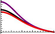
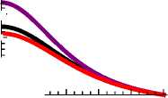
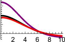
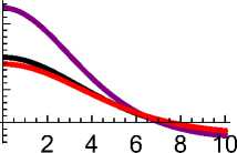
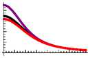
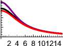
The evolution of energy density and pressure components is crucial for verifying the viability of the constructed models. Figure 1 shows the energy density profile p(r) for different compact star candidates, highlighting that p reaches its maximum value at the center ( r = 0 ) and monotonically decreases with radial distance. This behavior is consistent with the expectations for realistic stellar models, where matter is densest at the core and becomes more dilute outward. The higher central density also reflects the ultra-compact nature of strange stars.

Model 1 ^ρ

Model 2

0.08

0.06

0.04

0.02

2 4 6 8 10

CS1

CS2

CS3

r

ρ

0.08

0.06

0.04

0.02

2 4 6 8 10

CS1

CS2

CS3

r

Fig. 1. Energy density profile for HerX - 1, SAXJ 1808.4“3658, and 4U1820“30 for two distinct f (R) gravity models. The plot indicates a decreasing density from core to the surface, confirming high compactness and regular matter distribution.

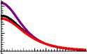
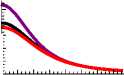
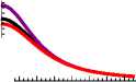
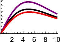
Similarly, Figures 2 and 3 display the behavior of radial pressure p r and transverse pressure p t , respectively. Both pressures are maximum at the core and decrease outward, which is a typical requirement for hydrostatic equilibrium in anisotropic configurations. These profiles are essential for understanding how internal forces maintain stellar stability against gravitational collapse.

Model 1

pr

Model 2

0.015

0.010

0.005

0.000

CS1

CS2

CS3

pr

0.015

0.010

0.005

0.000

CS1

CS2

CS3 r

Fig. 2. Radial pressure evolution for HerX — 1, SAXJ 1808.4“3658, and 4U1820“30 under two f (R) models. The monotonic decrease from the core to the surface reflects consistent behavior with physically viable stellar models.

Model 1

Model 2

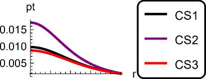
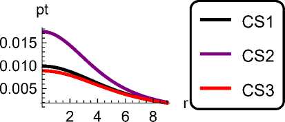
Fig. 3. Transverse pressure evolution for HerX — 1, SAXJ 1808.4“3658, and 4U1820“30 for two different f (R) gravity models. The pressure is higher near the core and decreases outward, contributing to the anisotropy factor in the stellar interior.

Radial Derivatives of Physical Quantities

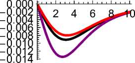
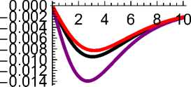
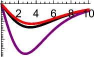
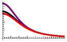
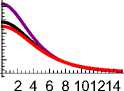
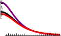
To further investigate the internal structure and validate the physical acceptability of the models, we examine the derivatives of the energy density and pressures. Figures 4, 5, and 6 show that dp <  0 , dp r <  0 , and dp- <  0 , indicating decreasing functions with radial distance.

At the center ( r = 0 ), the following conditions are satisfied:

dρ dr

r =0

= 0,

dp _r dr

r =0

= 0,

dp t dr

=0

r =0

These conditions are physically required to ensure the regularity and finiteness of thermodynamical quantities at the core. Additionally, the observed monotonic decrease of density and pressure with increasing radius is a strong indicator of the physical plausibility of our models in the Finch-Skea framework.

Model 1

Model 2

d p/dr

CS1

CS2

CS3

d p/dr

CS1

CS2

CS3

Fig. 4. Radial derivative of energy density for HerX — 1, SAXJ 1808.4“3658, and 4U1820“30 under two f (R) models. The decreasing trend confirms a realistic matter distribution where density decreases from core to surface.

Model 1

Model 2

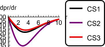
Fig. 5. Radial derivative of the radial pressure for HerX — 1, SAXJ 1808.4“3658, and 4U1820“30. The negative gradient ensures proper hydrostatic balance required for equilibrium.

Model 1

Model 2

dpt/dr

0.0000

-0.0005

-0.0010

-0.0015

-0.0020

-0.0025

CS1

CS2

CS3

dpt/dr

0.0000

-0.0005

-0.0010

-0.0015

-0.0020

-0.0025

CS1

CS2

CS3

Fig. 6. Radial derivative of the transverse pressure for He'rX — 1, SAXJ 1808.4“3658, and 4U1820“30. The decreasing trend supports regularity and anisotropy decay in stellar interiors.

Energy Conditions

The energy conditions are important criteria for ensuring the physical viability of energy-momentum tensors in gravitational theories. Derived from the Raychaudhuri equation [53, 54], they express conditions under which gravity retains its attractive nature and matter behaves in accordance with relativistic causality [55]. In the context of anisotropic compact stars in f (R) gravity, we examine the following standard energy conditions:

• • Null Energy Condition (NEC):   p + p r >  0 , p + p t >  0

• • Weak Energy Condition (WEC):   p >  0 , p + p r >  0 , p + p t >  0

• • Strong Energy Condition (SEC):   p + p r >  0 , p + p t >  0 ,   p + p r + 2p _t >  0

• • Dominant Energy Condition (DEC):   ρ ≥ | p _r | , ρ ≥ | p _t |

0.08 0.06 0.04 0.02 0.00

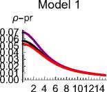
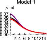
Our obtained models satisfy all the above conditions throughout the stellar configuration. Figures 7 and 8 illustrate the energy condition profiles for the two distinct f (R) models, confirming the physical reliability of the matter distribution in all three compact star candidates.

ρ+pr

Model 1 ^ρ

CS1

CS2

CS3 r

2 4 6 8 101214

Model 1

0.10

0.08

0.06

0.04

0.02

0.00

CS1

CS2

CS3 r

Model 1 ρ+pt 0.10 0.08 0.06 0.04 0.02 0.00

z

CS1

CS2

CS3 r

Model 1

p+pr+pt

0.12

0.10

0.08

0.06

0.04

0.02

0.00

2 4 6 8 101214

CS1

CS2

CS3 r

CS1

CS2

CS3 r

2 4 6 8 101214

CS1

CS2

CS3 r

Fig. 7. Energy condition verification for strange stars under Model 1: NEC, WEC, SEC, and DEC are satisfied across the radius for HerX — 1, SAXJ 1808.4“3658, and 4U1820“30.

Model 2

0.08

0.06

0.04

0.02

0.00

2 4 6 8 101214

Z            '

CS1

CS2

CS3 r

ρ+pr

0.00

Model 2

0.10

0.08 0.06

0.04

0.02

2 4 6 8 101214

■-------------------------------

CS1

CS2

CS3

r

ρ+pt

Model 2

0.10

0.08

0.06

0.04

0.02

0.00

2 4 6 8 101214

CS1

CS2

CS3 r

Model 2

p+pr+pt

0.12

0.10

0.08

0.06

0.04

0.02

0.00

2 4 6 8 101214

’-------------------------------■

CS1

CS2

CS3

r

Model 2

p-pr

0.06

0.04

0.02

0.00

■-------------------------------

CS1

CS2

CS3

r

Model 2 p-pt

0.06

0.04

0.02

0.00

2 4 6 8 101214

CS1

CS2

CS3 r

Fig. 8. Energy condition verification for strange stars under Model 2: The plots show that the models are physically viable and respect energy conditions throughout the interior.

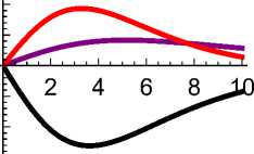
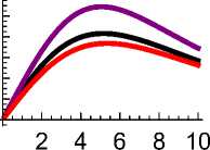
Tolman-Oppenheimer-Volkoff (TOV) Equation

To ensure equilibrium of self-gravitating systems, the Tolman-Oppenheimer-Volkoff (TOV) equation provides a balance between internal pressure gradients, gravitational attraction, and anisotropic stresses. In generalized anisotropic systems, the Tolman-Oppenheimer-Volkoff (TOV) equation [56, 57] takes the form:

dP r . a            ²⁽P r - P t )

~r^ + ^^p + p r ^{) +} —r—

= 0

This can be recast into the sum of three forces:

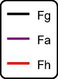
F g + F h + F a = 0,

where the individual forces are defined as:

_ _ BVCr(p _r + p)      _ dp r _ 2(p t - p r )

g A + 2 B^Cr² , h dr’ ^a r

Figure 9 displays the equilibrium profile, showing the interplay between the gravitational pull, hydrostatic pressure gradient, and anisotropic stress for three different compact stars under both f (R) models.

Model 1

Model 2

0.002

0.001

0.000

-0.001

-0.002

0.002

0.001

0.000

-0.001

-0.002

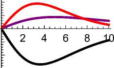
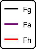
Fig. 9. Profiles of gravitational force (F g ), hydrostatic force (F h ), and anisotropic force (F a ) as functions of the radial coordinate r for HerX — 1, SAXJ 1808.4“3658, and 4U1820“30. Left panels represent Model 1, right panels Model 2. The net force vanishing confirms static equilibrium.

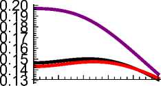
Stability Analysis

To investigate stability, we examine the radial and transverse sound speeds defined by:

₂     dp _{r     2}

v ^sr = dp ’    v ^st

dp t dρ

For causal and stable configurations, both speeds must lie within the interval 0 <  v 2 <  1 . Figures 10

and 11 show the variation of these sound speeds across the stellar interior.

Model 1

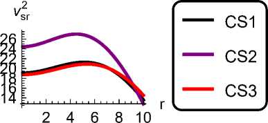
Fig. 10. Variation of the radial sound speed v _s ² _r with radial distance for the three strange star candidates. The speed remains within the causal bound 0 <  v 2 _r <  1 throughout the star.

Model 2

To ensure further stability, the Herrera cracking (or overturning) condition is also checked via the absolute difference |vs2t - vs2r |, which should remain less than 1.

Model 1

v s²t

0.20

0.18

0.16

0.14

2 4 6 8 10

CS1

CS2

CS3

r

Model 2

v s2t	CS1
0.20
0.18	CS2
0.16
0.14	CS3
0.12                     r

r

2 4 6 8 10

as a function of radial distance for the three compact

Fig. 11. Variation of the transverse sound speed v 2 _t stars. The models satisfy the causality condition.

Model 1

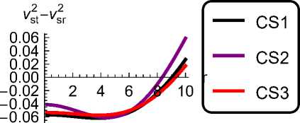
Model 2

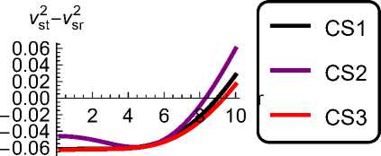
Fig. 12. Profile of Iv 2 _t — v 2 _r | with radius. The condition 0 <  Iv 2 _t — v 2 _r | < 1 is satisfied, confirming stability against cracking for all three star candidates in both models.

Equation of State (EoS) Parameters

For anisotropic matter, the equation of state parameters are given as:

Pr = Wrp, pt = wtp where wr and wt are the radial and tangential EoS parameters, respectively. For ordinary matter, the condition 0 < wr,t < 1 should hold, implying that pressure is positive and subluminal.

Model 1

Model 2

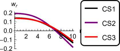
Fig. 13. Radial EoS parameter w _r = p _r /p as a function of radius for the three strange stars. The parameter

stays within the physical bounds 0 < w _r <  1.

Anisotropy Measurement

The anisotropy factor A quantifies the difference between radial and tangential pressures and is defined by:

A = ²⁽ P t - P r )

r

A positive value of A indicates that the anisotropic force is directed outward, which helps counteract the gravitational pull and supports higher mass configurations.

Model 1

wt

2 4 6 8 10

CS1

CS2

CS3

r

Model 2

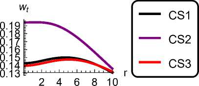
Fig. 14. Tangential EoS parameter w t = p t /p plotted across the radial coordinate. The condition 0 < w t < 1 is satisfied for all models.

Model 1

Δ

Model 2

0.0010

0.0008

0.0006

0.0004

0.0002

0.0000

CS1

CS2

CS3

r

Δ

0.0012

0.0010

0.0008

0.0006

0.0004

0.0002

0.0000

CS1

CS2

CS3

r

Fig. 15. Anisotropy parameter △ as a function of the radial coordinate. The positive trend ( △ > 0) suggests outward-directed anisotropic force, enhancing the stability and mass-bearing capability of the stars.

Conclusion

In this study, stable compact star configurations with anisotropic matter distribution have been investigated within the framework of f (R) gravity, where R denotes the Ricci scalar. The assumed stellar geometry is static and spherically symmetric, and it is modeled using the Finch–Skea spacetime, which satisfies the necessary junction conditions at the boundary surface. The constants in the metric functions are determined using physically realistic mass and radius values, making the solution applicable to various stellar models.

The primary goal of this work is to explore how modifications in the gravitational action via higher-order curvature terms affect the internal structure and stability of compact stellar objects. For this purpose, two well-established f (R) gravity models—one quadratic and one exponential in the Ricci scalar—are considered. These models extend the earlier analysis by Astashenok et al. [58], where it was shown that modified gravity can allow larger neutron star masses, particularly when realistic equations of state (EoS) are incorporated.

Figure 1 illustrates the inverse relationship between the radial coordinate and energy density: as r increases, the energy density decreases, suggesting a denser core region consistent with physically realistic stars. Figure 2 indicates that the radial pressure gradient ^d _d ^P _r ^r transitions from negative to positive, implying a local pressure minimum and highlighting the compact nature of the object. Similar trends are observed for the tangential pressure gradient ^d _d ^P _r ^t .

Figures 3–5 confirm that all energy conditions—Null, Weak, Strong, and Dominant—are satisfied throughout the star, supporting the physical viability of the matter configuration. In Figure 6, the Tolman–Oppenheimer–Volkoff (TOV) equation is used to analyze hydrostatic equilibrium. The gravitational force is shown to balance the anisotropic and hydrostatic forces, indicating a stable configuration under equilibrium conditions.

Figures 7 and 8 analyze the stability through the sound speed criteria. The squared speeds of radial ( v 2 _r ) and transverse ( v 2 _t ) sound waves remain within the causal range [0,1] for all configurations.

Additionally, the condition 0 <  | v 2 _t — v 2 _r | < 1 is fulfilled, ensuring that no instability due to cracking occurs.

Figure 9 presents the behavior of the equation of state parameter w _t = Pp t , which lies within the physically admissible range [0,1] , confirming a well-behaved tangential pressure profile. In Figure 10, the anisotropy measure A = P t — P r is shown to be positive in most of the interior region, indicating that the tangential pressure dominates the radial one. This repulsive anisotropic force allows for more compact and massive configurations.

The negative values of radial gradients in energy density and pressure reflect typical profiles of realistic neutron stars. The analysis also confirms that the matter distribution remains physically acceptable across the interior and that the Finch–Skea geometry can be effectively used to model compact stars in f (R) gravity.

Overall, our investigation emphasizes that the inclusion of higher-order curvature corrections in gravitational theory significantly influences the structural and stability features of stellar configurations. This work encourages further research into more generalized modified gravity theories and their relevance to astrophysical phenomena, especially in regimes where general relativity may face observational limitations.