Звукоизлучение вращающегося источника

Electronic Journal «Technical Acoustics»

For a helicopter or centrifugal fans, the noise generated from moving sources is usually very important. They are many kinds of aerodynamic noise including turbine jet noise, impulsive noise due to unsteady flow around wings and rotors. Accurate prediction of noise mechanisms is essential in order to be able to control or modify them to comply with noise regulations and achieve noise reductions. Both theoretical and experimental studies are being conducted to understand the basic noise mechanisms. The first integral approach for acoustic propagation is the acoustic analogy [1]. In the acoustic analogy, the governing Navier-Stokes equations are rearranged to be in wave-type form. The far-field sound pressure is then given in terms of a volume integral over the domain containing the sound source. However the major difficulty with the acoustic analogy is that the sound source is not compact in supersonic flows. The Ffowcs Williams and Hawkings (FW-H) equation [2] is introduced to extend acoustic analogy in the case of surfaces. However, when acoustic sources are presented in the flowfield, volume integration is needed. This volume integration of the quadrupole source term is difficult to compute and is usually neglected in most acoustic analogy codes. Errors can be encountered in calculating the sound field. Recently, there have been some successful attempts in evaluating this term.

Another alternative is the Kirchhoff method [3] which assumes that the sound transmission is governed by the simple wave equation. Kirchhoff’s method consists in the calculation of the nonlinear near- and mid-field, usually numerically, with the far-field solutions found from a linear Kirchhoff formulation evaluated on a control surface surrounding the nonlinear-field. The control surface is assumed to enclose all the nonlinear flow effects and noise sources. The sound pressure can be obtained in terms of a surface integral of the surface pressure and its normal and time derivatives. This approach has the potential to overcome some of the difficulties associated with the traditional acoustic analogy approach. The method is simple and accurate and accounts for the nonlinear quadrupole noise in the far-field. Full diffraction and focusing effects are included while eliminating the propagation of the reactive near-field.

More experimental studies to the complexity of sound generation of moving sound sources have been presented. In 1965, M. V. Lowson [5] derives firstly acoustic field equations produced from rotating point force. The equations are applied successful to predict the sound radiation of rotors. The sound field mechanism of the linear motion point source with the moving coordinate system is first proposed by P. M. Morse [4] in 1968. The sound radiation equations are only available for simple moving point sources and the method of coordinate transform is difficult for the complex motion sources. The equations are only used to predict the moving sources in free field. However, in most applications only a few locations are needed to study directivity and compare with measurements. Also, for many numerical solution of field equations dissipation and dispersion errors and an accurate description of propagating far-field waves is compromised. Sound field equations of rotating point force with cylindrical boundary using direct boundary element method have been deduced by K. D. Ih and D. J. Lee [6]. Helmholtz equation and its normal derivative of moving surface are given. The equations are applied to discuss the sound source’s types and are extended to explore acoustic radiation of centrifugal fans by W. H. Jeon and D. J. Lee [7–10]. These methods have established the foundation for sound radiation of moving source but there are some problems needed to overcome further. First the simplification of the fact with the assumption of point source and plane wave will bring more inaccurate for the prediction. Second, the sound pressure equations are often given in time domain. The time models are difficult to calculate and obtain the numerical solution.

In order to deal with the problems, sound radiation in frequency domain is investigated in the paper. The analytical expressions of the pressure of rotating monopole and dipole based on numerical Green function are derived. Characteristics of sound field are explored by numerical simulation. The analytical method provides important theoretical value for the research of sound radiation and noise control of moving source.

• 1 . ANALYTICAL FORMULAE

In this section, the analytical Green function and sound pressure model of rotating compact sources are derived in frequency domain. The Green formula is as a common starting point.

• 1.1 . Free-field analytical Green function

  • 1.1.1    Rotating point source

The Green function G ( x , y , t, т ) is defined as the response of the flow to an impulsive point source represented by delta functions of space and time. G ( x , y , t , т ) is the acoustical response measured in x at time t of a source placed in y fired at time т :

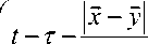
I^ -V ^{2 G} = $ ( ^x - y ) $ ( t - т ) .

where 6 ( x - y ) = $ ( x 1 - y 1 ) 6 ( x ₂ - y ₂ ) $ ( x 3 - y 3 ) , when t < т , then G = 0 .

G ( x , y , t , т ) =

-----i--------Г $

4 n|x - y|

к c 0 7

4 n r s

r

$ t - т - s к         c 0 7

where c ₀ is the sound speed.

Introducing G ^ˆ as shorthand notation for the Fourier transform of Green function, which is defined by

G = — Go G ( x , y , t , т ) e ^iMdt .

2 n

Taking the Fourier transform on both sides of the formula (2) then Green function in frequency-domain can be deduced:

, ,      \       1      - i a t i K r

G (x, y, а, т )= e e s , 8n2 rs where a is the frequency, к = а / c0 is wave number.

Rotating point source configuration is in figure 1. Location of initial point source is ( r , 0 , ^ ) , observation location is ( r ₀, 0 ₀, ^ ₀ ) , where ^ = ^ т , 0 = я/ 2, Q are the rotating angular frequencies.

In the spherical coordinate, we expand the term e k /4 л r of formula (3) with Legendre and spherical harmonic functions:

k s

T- = i K X b n X Y" ’ (^ )Y : ( « . • ? . ) = f Z (2 ” + 1) bP (cos в ).                  (4)

‘nr      ,= 0 m =-,                        4 n , = 0

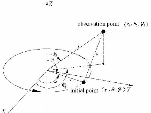
Figure 1. Rotating point source

By the Euler's formula and addition theorem:

n

P, (cos в ) = у g m a m.. [ e m (' ^-" °' m = 0

n

+ e - m(' -®o) J = у g a  [ emo e - m ^t + e - mo emПт J m=0

where b_n

< jn ( K ro)h n ( ^K r ) . jn ^{( K} r) ^hn ( ^K r 0 )

r >  r o

r <  r o

(1/2 m = o         (n - m)! mm          m sm "{1 m = 1-n, amn   (n + m)! Pn (COS^)Pn (cos6,°)’

в is the angle between the vector r _o and r.

Green function of rotating point source in free space is given by

^ n

G ( x , y, "T ) =     УУ g m ( 2 n + 1 ) Ь^ ( e -i" ' J" ⁺ ’ " + e^ e i ⁽" ^- m *) .               (5)

^{8 n} n = o m = o

• 1.1.2    Rotating dipole source

Rotating dipole source’s analytical Green function and sound field expressions in frequency domain are derived. They are two different types dipole, the horizontal (along the ' orientation) and vertical directions (along the z axis), are discussed. They are shown in figure 2 and 3 respectively.

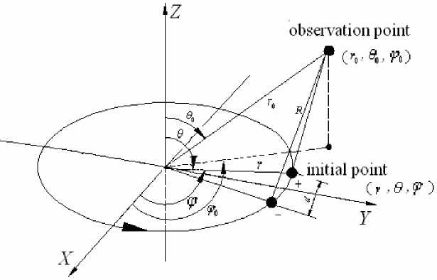
Figure 2. Horizontal rotating dipole source

z observation point

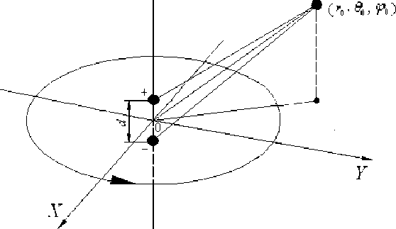
Figure 3. Vertical rotating dipole source

We can get multipole Green function by the partial derivatives of source coordinates of rotating point source’s Green function. Vertical Green function of dipole source is defined by the derivative of G along the source coordinate Z ( в = 0 ) :

Л              Лzv

G z = -d G / d z = - ( d G / d r ) cos в ,

G, (r/ r) = tt ■ (-К2)["’n ' 1) 1 cosвЬ',a (e ^ e-'“*ma)' + em”e-(“—ma)'),(7)

n=0 m=0            \ 8n/ where b'n

jn ( ^{K r} 0 ) h ‘ ( ^{K r} )

Jn ^{( K r} ) h n ( ^{K r}0 )

^r >  ^r 0 ,

^r <  ^r 0 -

л

Horizontal Green function of dipole source is the derivative of G along the p orientation:

Л.

TV

G p

X dG r0

v(2 n ⁺

^G p ( r / ^r 0 ) = L ⁽ - ^{i K} / ^r 0 ^)[^^^] b n *

n=0

< P_n ( 0 ) P_n ( 3 ) - L ⁽ n — m ^{) !} P_n^m ( 0 ) P nm ( 3 ) im Г e^{im p} 0 e i ^{( a + m Q T} - e 'm ^p e i ^{( a} - ^{m q ) t} 1 > .

Z1 (n + m)!                   L1

• 1.2    Sound pressure model and directivity

  • 1.2.1    Sound pressure of rotating dipole source

We assume that the acoustic field is from a given time-harmonic source distribution

Q s ( t ) = Q ( t ) e - "' , then the sound pressure is given by

p(r, t )=L Qs (t )GdT=t Qs (t) 41^ ^( t- T - RJdT(9)

Taking the Fourier transform on both sides of the formula (9) then we can get sound pressure in frequency-domain:

1 f^ f^1 Г^

p(r, a) = — [ Г Qs (t) Ge" drdt = — I Q(t)e" iaTGdr,(10)

2 n ^J-“^J- “                     2 n ^J-“

Q ( t ) is point source strength. We define the dipole strength D_s = Q_sd and assume that d is vanishingly small and the A 0 ( a ) is the Fourier transform of Q ( t ) , then

A (a) = 2П-CQT’e-i"'dT'(11)

For a given time-harmonic source, formula (11) is rewritten as

A (a) = QS(®- щ), where at is the source vibration frequency (nature frequency). The sound pressure of rotating dipole source is presented P.

^Pz = ^Ds ЕЁ ^£ m ^{( - i K 2} ) f ⁽² n ^{+ 1) J cos 3} 0 B n ⁽ n , m ) ! * ^Pm ( ⁰ ) ^Pnm ( ^{cos 3} 0 ) * Г ( e im ^{(- P} 0 B ( ^{a + m Q} - Щ ) )

n=0 m=0          \ 8n )         (n + m ’!

+ (e -im (-p0 ’B(a - mQ- at)’], co

- K (2 n + 1) B_n 8 n² r ₀

■ P n ( 0 ) P n ( cos 3 ₀ ) - Ё im ( n—m ) | P nm ( 0 ) P nm ( cos 3 ₀ ) * [                     m = 1 ( n + m ) !

( e m ( ^p 0’ B ( a + m Q- a _t ) + e im ^{( p} ’ B ( a - m Q- a _t ) ) } .

• 1.2.2    Directivity of rotating dipole source

The far-field directivity pattern is defined by removing the e^lKr/r factor so that the directivity pattern D (в , ^ ) is defined by

J “[ P ( r , в , ^ ) ] = ( ^e ^‘"r/ r ) D ( в , ^ ) .                                                         (15)

Far-field directivity of rotating dipole source:

D z ( в , ^ ) = re -r P , D ^ ( в , ^ ) = re ^{- i K r}P _v .                                                    (16)

• 2    NUMERICAL ANALYSIS OF SOUND FIELD

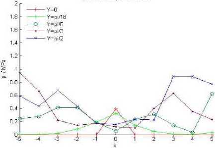
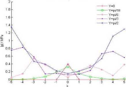
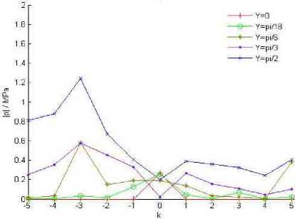
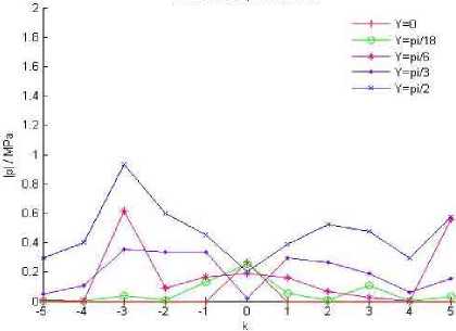
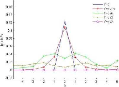
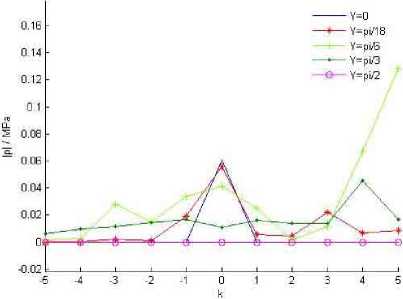
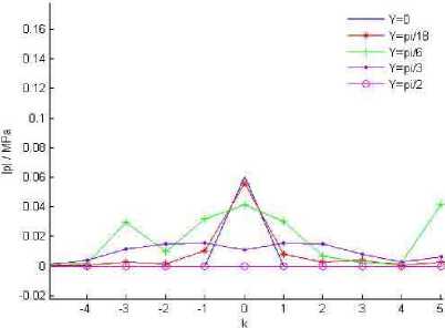
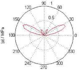
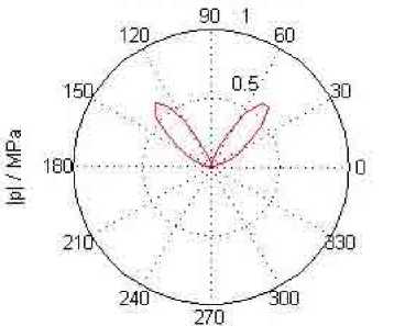
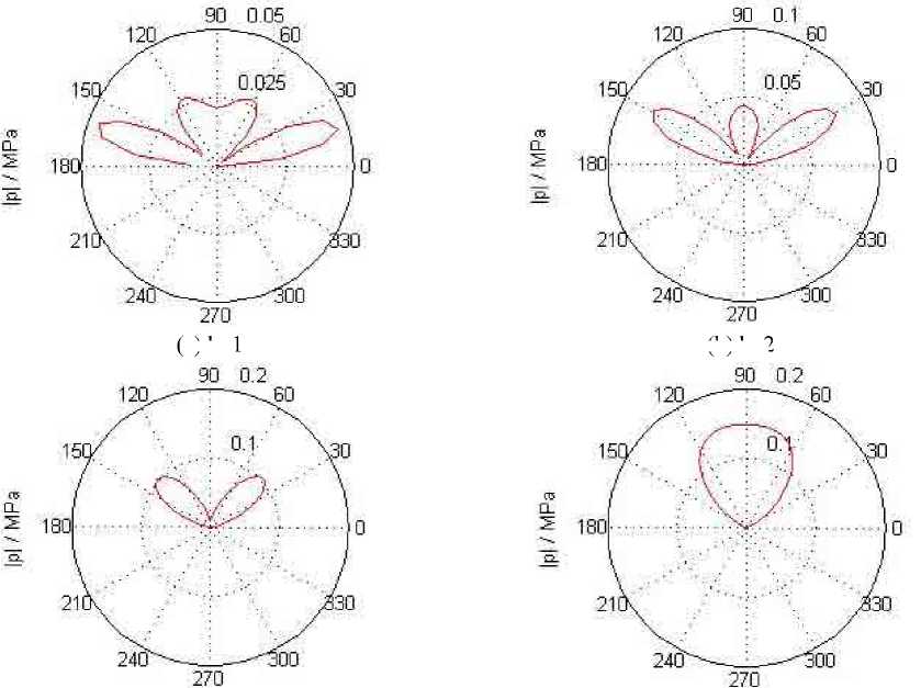
  Acoustic field characteristics are given in the condition of time-harmonic source. Simulation parameters: azimuth of observation point ^ 0 = n /4, source nature frequencies a t are 2300 and 6800 Hz, rotating angular frequencies Q are 112 and 560 rad/s, acoustic field frequencies are shown by a = a t + k Q . k is harmonic orders and is for integer k = - 5,---,5. Observation angle в ₀ are given 0, n /18, n /6, n /3, n /2 . For far-field r = 2 m and r₀ = 0.3 m . Simulation results are demonstrated from figure 4 to figure 7.

(a) a t =6800 Hz, a ₀ =560 rad/s

(b) a t =6800 Hz, a ₀ =112 rad/s

(c) a t =2300 Hz, a ₀ =560 rad/s

Figure 4. Sound pressure amplitude distribution of vertical dipole with observation angle at different nature and angular frequencies

(d) a t =2300 Hz, a ₀ =112 rad/s

With the increasing of nature frequencies, the far-field sound pressure amplitude of vertical dipole increases, the scope of harmonic distribution expand and fundamental frequency component reduce with the observation angle augmentation. Harmonic distribution is the most abundant in the observation angle of π /2. There is only fundamental frequency in the rotating axis direction. With the increasing of angular frequencies, the distribution of harmonics and sound pressure amplitude increase. Doppler frequency shift phenomena are appear clearly with higher angular frequency shown in figure 5.

(a) Low Frequencies

(b) High Frequencies

(a) ω _t =6800 Hz, ω ₀ =560 rad/s

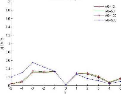
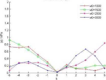
Figure 5. Sound pressure amplitude distribution of vertical dipole with different angular frequencies at 60 ° observation angle

(c) ω _t =2300 Hz, ω ₀ =560 rad/s

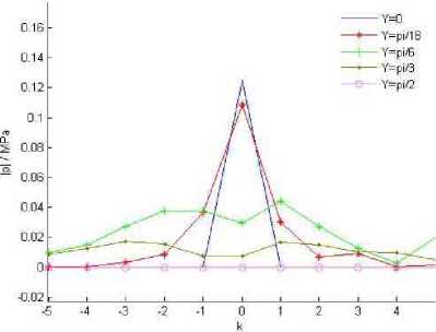
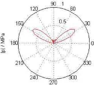
Figure 6. Sound pressure amplitude distribution of horizontal dipole with observation angle at different nature and angular frequencies

(b) ω _t =6800 Hz, ω ₀ =112 rad/s

(d) ω _t =2300 Hz, ω ₀ =112 rad/s

Sound pressure amplitude is impacted greatly by the nature frequencies. The scope of harmonic distribution expands with the increasing of view angle in figure 6. Fundamental frequency is evidence in the small observation angle as 0 and π /18. There are no harmonic orders in the observation angle π /2. The nature and angular frequencies changing have great effect on the harmonic distribution.

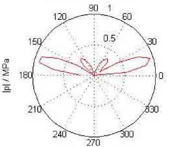
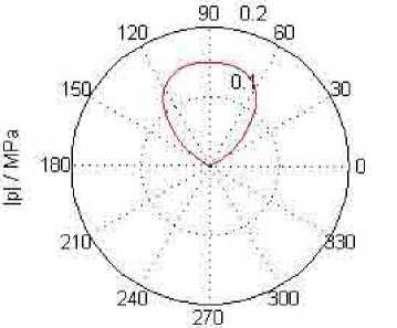
Rotating dipole source have an intensive space directivity which is shown in figure 7 and figure 8.

(a) k=1

(b) k=2

(c) k=3

(d) k=5

Figure 7. The directivity of vertical dipole with different harmonic orders at the same and

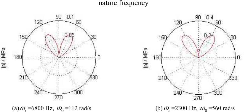
Figure 8. The directivity of vertical dipole with different nature and angular frequencies at

harmonic order k=5

With the increasing of harmonic orders, the directivity of vertical dipole becomes intensive. Especially, sound power focuses on the range from π /6 to π /3 in figure 7. The changes of nature and angular frequency have a small effect on the directivity of vertical dipole. It is shown in figure 8.

(a) k=1

(b) k=2

(c) k=3

(d) k=5

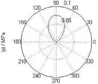
Figure 9. The directivity of horizontal dipole with different harmonic orders at same nature and nature frequency

(a) ω _t =6800Hz, ω ₀ =112rad/s

(b) ω _t =2300Hz, ω ₀ =560rad/s

Figure 10. The directivity of horizontal dipole with different nature and angular frequencies at harmonic order k=5

With the increasing of harmonic orders, the directivity of horizontal dipole becomes intensive. Especially, sound power focuses on the range from π /3 to π /2 in figure 9. The change of nature and angular frequency has a small effect on the directivity of horizontal dipole. It is shown in figure 10.

CONCLUSIONS

A frequency-domain method has been developed for prediction of sound field of rotating diople source. The method is based on the acoustic solution of rotating point source in freqency-domain with analytical Green function. Solutions are carried out employing an explicit sound pressure model and the characteristics of sound field of moving source. By numerical simulations we can get that the sound field frequency involves nature frequency, angular frequency and its harmonics. With the increasing of nature and angular frequency, sound field radiation frequency becomes complex. The free-space directivity of rotating source is intensive greatly. The method and results have important theoretical significance on the moving source sound field characteristics analysis and exploring the low-noise design of rotary machines.