A model for estimating firmware execution time taking into account peripheral behavior

Published Online June 2018 in MECS

Nowadays, the market of real-time embedded systems is constantly growing. Thus, in order to keep up with the market, one needs to speed up the process of bringing out each new release of a real-time embedded system [1, 2]. Consequently, it raises the need to intensify all the production processes including quality assurance procedures. All this testifies the importance of reliable, time-efficient, automated tools for quality assurance of both software and hardware components of real-time embedded systems.

In hard real-time systems, each time-critical activity should meet its deadline. However, any firmware execution time depends not only on the microcontroller itself but also on peripheral devices connected to it.

Moreover, the latter can be inclined to more or less uncertainty in their response. Depending on their type, model and the time of being in use, i.e., when a peripheral device wears out, its characteristics make their operation slower in general and their behaviors become less determined. In order to evaluate the firmware’s execution time, they use the following metrics: worst-case execution time (WCET) [3, 4], best-case execution time (BCET) [5, 6] and average-case execution time, (ACET) [7, 8]. The latter resides within the interval [BCET -WCET] and depends on the distribution of the program execution time. The narrower the above-mentioned range, the less uncertainty we have to deal with, and a slow high-predictable system might be preferable than a fast unpredictable one. Despite the fact there exist different methods and techniques for execution time estimation, they all ignore the influence of hardware components on the total execution time [9-22]. However, hardware components not only contribute to the total delay, they also posse a great deal of uncertainty which is to be measured and taken into account.

From the point of view of its users, a system should perform some actions within an expected time period. From the embedded software engineers’ slant, each of such activities is performed by a set of functions in firmware and the total predictability of each activity is determined by the weakest item among these functions. A model allows embedded software engineers to evaluate the predictability of execution time for each function in firmware and thus detects the weakest items in their systems might be of significant importance in the testing and maintenance stages of the system’s life cycle. First, as mentioned above, any hardware component is prone to get less predictable over-time and inspection of the existing embedded system by using the model, it allows us to detect and to replace hardware items that contribute most uncertainty to the whole system. Second, the system might be ported to another, newer and more advantageous hardware platform while its main application logic should be preserved. The model allows us to avoid an erroneous choice of hardware components reducing the predictability of the execution time of the system’s time- critical functions. Moreover, since there is time limitation for any project and any single stage, the model is helpful for quality assurance engineers when they plan their activities (here, we assume that less determined functions require more attention).The work is aimed at developing and verifying a model for evaluating the predictability of the execution time of all the functions in a system and a software tool based on this model.

This paper is organized as follows: a proposed model is presented in section II. The process of verification of the proposed model that had been conducted on a real embedded system is described in section III. A conclusion and future work is suggested in section VI.

• II.    A Model for Estimation of Embedded Systems’ Code Execution Time

We divide all the instructions in the firmware into two groups: 1) those dependent only on the microcontroller itself and 2) those dependent on peripheral devices. Thus, the execution time of any function will have its more or less stable component and a variable component influenced by hardware.

Step 1 . The first stage assumes the syntax analysis of the whole system performed using the map-file generated during firmware compilation. The names of all the functions are placed into the dedicated table in a database, the structure of which is represented by Table 1.

Step 2 . All the instructions of the first group written in a high-level language come down to a set of assemblerlike instructions. The latter depends on the microcontroller and an IDE keeps its database of the microcontrollers. The database suggests which instructions are used to transform any hi-level code. In RISC microcontrollers, each instruction typically takes one clock pulse to be executed, an instruction may take 1 to 12 clock pulses in CISC. Using IDE’s capabilities, one may find out which assembler-like instructions represent each high-level instruction. For example, Fig. 1 shows how such a correspondence is provided by IDE Keil uVision for a code written in C, the instructions for microcontroller STM32F205.

At this stage, the total duration of all the hi-level instructions contained inside the function being evaluated should be calculated. I.e. the algorithm starts with the function beginning, parses the information about the correspondence between its high-level and assembler-like instructions and counts the total duration of the latter. I.e., the algorithm selects all distinct function names from Table 1. Each function iteratively searches name in all the listing files for all the references to this name. Among these references, only one will be the function’s body, all the others are just invocations. The body of any function starts with PUSH and ends with POP in the assemblerlike code and this fact can be used to recognize the first and last instruction in the assembler-like representation of a function. During the phase of compilation, an IDE creates as many listing files as many .c files in the project under compilation. The set of instructions supported by each microcontroller is available from its programming manual; it’s convenient to keep this data in a separate table in the database as shown in Table 3. As the result of this stage, Table 1 is appended by two values per function – the possible total duration of all the minimum microcontroller-dependent instructions in the function being analyzed and the corresponding maximum value.

The need of keeping two values instead of one is attributed to the fact that the clock frequency might not be perfectly stable. It depends on the clock generator selected (quartz generators are the most accurate whereas RC circuits are generally inferior to them in accuracy). Thus, the minimum stable execution time is the result T of counting the total duration of all the relevant assembler-like instructions minus N% of the clock frequency, whereas the maximum stable execution time is equal to T + N%.

Step 3 . Next, we evaluate the range of random execution time for each hardware-dependent instruction.

Typically, the code of an embedded system contains parts like this:

while() {}; /* a blocking condition needed because the next instruction simply does not make sense without the result of the previous action */

Table 1. The table for storing the main results of execution time estimation

Function Name	Branch Number	Min. Stable, s	Max. Stable, s	Mean Value, s	Mean – Variance, s	Mean + Variance, s
main	Branch 1	3.676·10-7	4.063·10-7	0	0	0
FlashDataRead	Branch 1	1.244·10-7	1.375·10-7	0	0	0
FlashDataRead	Branch 2	1.979·10-7	2.188·10-7	1.166·10-4	·10-3	·10-3
FlashDataRead	Branch 3	2.714·10-7	3·10-7	2.332·10-4	·10-3	·10-3
FlashDataWrite	Branch 1	1.131·10-7	1.25·10-7	0	0	0
FlashDataWrite	Branch 2	1.866·10-7	2.063·10-7	1.166·10-4	1.1658672·10-4	1.1661328·10-4
FlashDataWrite	Branch 3	2.488·10-7	2.75·10-7	2.332·10-4	2.3314687·10-4	2.3325313·10-4
EraseSector	Branch 1	1.414·10-7	1.563·10-7	0	0	0
EraseSector	Branch 2	1.866·10-7	2.063·10-7	0.721	0.691	0.751
EraseFlash	Branch 1	1.696·10-3	1.875·10-3	0	0	0
EraseFlash	Branch 2	1.866·10-7	2.063·10-7	5.452	1.386	9.518

9	;;; 55	|int main (void)
10	000000	bS38	PUSH	(r3-rS,lr}
	;;; 56	{
	;;;57	int timl •	1;
13	000002	2001	MOVS	rO,«l
14	000004	9000	STR	rO,[sp,*OJ
IS	;;; 58	osStatus	status;
	:;:59
17	;;; 60	osKernellnj	Ltialize ();	// initialize CMSIS-RTOS
	000006	f7fffffe	BL	osKernellnitlallze
19	;;; 61	// initialize peripherals here
20	;;; 62	tid_HWSystesiInitTask =		osThreadCreate (osThread(HWSysten>InitTask), NULL)
	oooooa	2100	MOVS	rl,#0
22	00000c	4833	LDR	rO,I LI.2201
	OOOOOe	f7fffffe	dL	osThreadCreate
24	000012	4933	LDR	rl,|LI.2241
25	000014	6008	STR	rO,trl,*O] : tld_HWSystemInltTaak

Fig.1. A fragment of a Listing file showing the correspondence between C code and assembler-like code of function main

Waiting is implemented by a flag which is initially set to TRUE. The flag is a variable in the firmware that its value may changes when the state of the corresponding hardware component changes. Any change of state is reported to the microcontroller in different ways, for example, by polling the state of the corresponding pin, via an interrupt or via reading some RX (receiving buffer), etc.

There scarcely might be a situation when two different flags are used in the same condition of while. I.e., we can reasonably assume that every operator ‘ while ’ corresponds to no more than one hardware-dependent flag.

The idea is to track those of the flags (i.e. variables value of which are changed along with the state of hardware components) that are used in blocking conditions like that one presented above, and to collect all the information on them in a database table, the structure of which is reflected in Table 4. In order to obtain such a table, one should parse all the library files being in use in the project first. Besides, all the IRQ handlers should be parsed as well. Table 5 summarizes the correspondences between constructs with a random execution time, the flags and the corresponding hardware activity to be waited for. In order to evaluate the possible duration of the blocking conditions, we just represent them as a range [T1,T2] where T1 and T2 are the minima and maximum possible duration of the corresponding hardware activity.

Information about all the hardware delays can be found in the manual of a specific hardware component (an example is shown in Table 2).

It’s worth bearing in mind that any hardwaredependent instruction partially depends on the microcontroller itself. That’s why all the assembler-like instructions will be considered when the invariable part of the firmware execution time is analyzed no matter whether they are blocking conditions or not.

Step 4 . Let’s suppose that the function under evaluation contains M instructions with some time uncertainty, which are described by intervals [a1,a2], [b1,b2]…[x1, x2] (as shown in Fig. 2). We assumed that the duration of any hardware-dependent operation follows the Gaussian distribution and verified this assumption having conducted a range of experiments with a sample of random-time operations in real embedded systems. The results tended to be close to the mean value of the interval where each tested operation was supposed to be in accordance with its documentation

In order to evaluate the minimum and maximum values of the random component of the function’s execution time, Monte-Carlo method is applicable 【】 . It provides the accuracy 1/sqrt(N) where N is a number of numerical experiments performed. Number N should be big enough to enable us making any statistical conclusions.

Table 2. Part of AT45DB041D Flash-SPI’s documentation showing the minimum, maximum and typical duration of each operation

Symbol	Parameter	AT45DB041D (2.5V version)			AT45DB041D			Units
		Min.	Typ.	Max.	Min.	Typ.	Max.
t XFR	Page to Buffer Transfer Time			200			200	ms
t comp	Page to Buffer Compare Time			200			200	ms
t EP	Page Erase and programming time (256/264 bytes)		14	35		14	35	ms
t P	Page Programming Time		2	4		2	4	ms
t PE	Page Erase Time		13	32		13	32	ms
t BE	Block Erase Time		30	75		30	75	ms
t SE	Sector erase time		0.7	1.3		0.7	1.3	s
t CE	Chip erase		5	12		5	12	s
t RST	RESET pulse width	10			10			μs
t REC	RESET recovery time			1			1	μs

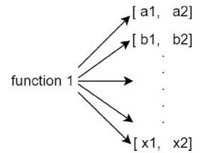
Fig.2. A list of time intervals representing uncertainty of the execution time of a function

At this step, each function should be considered again “from scratch” on the basis of the database Table 1 that have been already filled in.

For each function in the firmware being evaluated, a temporary table (the structure of which is shown in Table 6), should be populated with the intervals of values that each of the hardware flags influencing our function’s execution time might be assigned. Then the algorithm iteratively generates N sets of random values normally distributed inside the intervals [a1,a2], [b1,b2]…[x1, x2], and each iteration calculates the total function’s execution time (using the above mentioned constant components).

The mean value of all the numerical experiments characterizes the most probable value of the function execution time while the variance indicates the maximum value by which the execution time ξ in any single experiment may differ from the mean value.

1 N 1 ( N V

D ^ * — У( ^ )2 - - У ^ I (1) N - 1 N ( j )

Table 1 should be appended by the values Mean, (Mean – Variance) and (Mean + Variance).

In practice, instructions might possess some uncertainties in their execution time which are placed in parallel branches of the function code. Thus, there is a need to associate each instruction with a random execution time and the function’s branch to which the instruction belongs. This approach allows us to evaluate the execution time of each branch in a function separately and to define the branches that quality engineers should focus on most assiduously.

The model might give more accurate results if we take into account the probabilities of the conditions in conditional statements being true. That’s because some operation with great uncertainty in its execution time may be executed only under a very unlikely condition and thus have little influence on the total function’s execution time. In contrast, some less uncertain operation occurring frequently contributes as much or even more into the total uncertainty in the function’s execution time. For example, if cyclic redundancy code for the data retained in an EEPROM chip indicates data corruption, the whole chip should be rewritten [26]. This time-consuming operation slows down execution of the whole function but is not likely to be executed every day since data corruption normally does not take place so often. On the opposite, check on EEPROM chip’s presence is a comparatively fast operation with little uncertainty but it should take place every time when the embedded system is switched on.

In order to enhance the accuracy of the results, we evaluate the probabilities of all the conditions being true.

Step 5. Using SQL and the information accumulated in the database at the previous stages, one can figure out the dependencies between the functions with the least certain execution time and the hardware components they use. Moreover, one can detect the hardware components with the greatest relative contribution to the system’s behavior in general.

Table 3. Assembler instructions info list

Assembler Instruction	A number of cycles taken
MOVE	1
ADD	1
ADDS	1

Table 4. Hardware blocking condition list

File Name	Function Name	Row number	Flag Name
Init	HardwareInit	15	SPI_I2S_FL AG_TXE
MainLoop	MainLoopTask	45	SPI_I2S_FL AG_RXNE
Background	BackgrnTask	22	DMA_IT_T CIF0
Background	BackgrnTask	43	DMA_IT_T EIF0

Table 5. Hardware flags list

Flag Name	Hardware model/Operation type	Procedure
SPI_I2S_FLAG_TXE	AT45DB041D/ Write Buffer	Interrupt data send
SPI_I2S_FLAG_RXNE	AT45DB041D/ Read Buffer	Interrupt data receive
DMA_IT_TCIF0	Internal DAC/ Send data	Interrupt transfer complete
DMA_IT_TEIF0	Internal DAC/ Send data error	Interrupt transfer error

Table 6. Hardware response time

Hardware model	Operation type	Min response time, us	Max response time, us
LIS302_DL	Read register	20	200
AT45DB041D	Page erase	13000	32000
AT45DB041D	Block erase	30000	75000

The proposed algorithm is represented by its block diagram (Fig. 3). The module structure of a computer application for estimating firmware execution time is shown in Fig. 4.

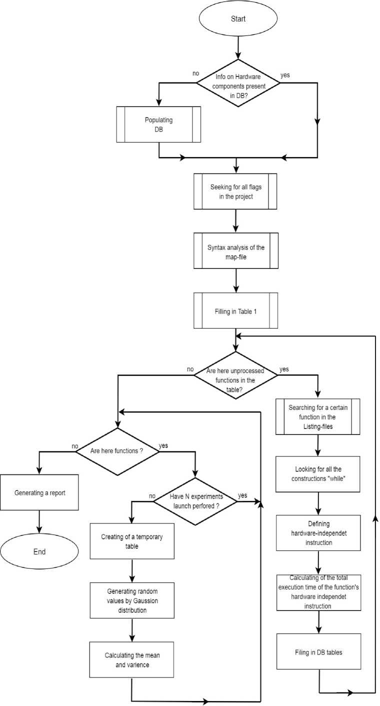
Fig.3. The block diagram of the proposed algorithm

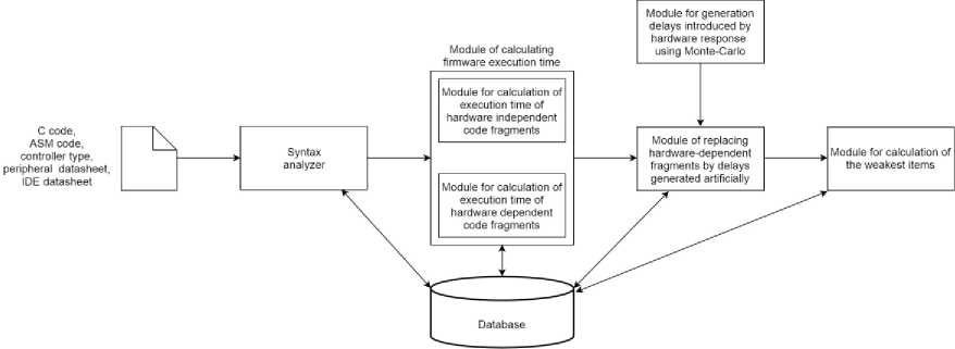
Fig.4. The module structure of the proposed computer application

• III.    Experiments

Verification of the proposed model has been performed in several stages.

At the first stage, a number of experiments were conducted on a real embedded system. We selected the functions from a project that depend on a response from hardware components more than other functions in the same project. The example of such functions is given below.

Code example //Input: Signal Flag void ReadTempAndPressTask (void const *argument)

{ osEvent evt;

float SampleBuffer[3][10];

float average[3];

short internal = 0;

short temp = 0;

short Chanel = 0;

byte i, j = 0;

byte Counter = 0;

for (;;)

{

/* The body of the loop itself executes each time when the thread is invoked by the operating system, however, no meaningful code is run until the thread receives the signal it’s waiting for. */ evt = osSignalWait(0x0001, osWaitForever);

{ /* once the desired signal is obtained, the following code is executed once and then the signal is automatically cleared */ for (Counter = 0; Counter < 10; Counter++)

• { /* here we get 10 samples of ADC readings */

  /* starting conversion using an internal ADC */

StartConversionOfInternalADC_1();

/* waiting until SPI gets free */ while(SPI_Get_Flag(SPI1, SPI_FLAG_BSY) == SET);

/* starting conversion using channel 1 of the ADC */ internal = ADS_Read(ADSCON_CH1);

/* starting conversion using channel 2 of the ADC */

Chanel = ADS_Read(ADSCON_CH2);

temp = Chanel + local_compensation(internal);

/* converting the value into the temperature */

SampleBuffer[0][Counter] = ADC_code2temp(temp);

/* waiting until SPI gets free */ while(SPI_Get_Flag(SPI1, SPI_FLAG_BSY) == SET);

/* starting conversion of data obtained from the internal temperature sensor */

Chanel = ADS_Read(ADSCON_INTERNAL);

temp = Chanel + local_compensation(internal);

/* converting the value into the temperature */ SampleBuffer[1][Counter] = ADC_code2temp(temp);

/* waiting for the flag “end of conversion” that is to be set by the internal ADC */ while(ADC_Get_Flag(ADC1, ADC_FLAG_EOC) == SET);

/* here we calculate the pressure value and put this value into a buffer */

SampleBuffer[2][Counter] = (GetPressure() / 100.0);

} for(i = 0; i < 10; i++)

{ for(j = 0; j < 3; j++)

{ average [i] += SampleBuffer[j][i];

}

}

/* averaging the measured values */ for(j = 0; j < 3; j++)

{ average [j] = (average [j] / 10);

}

/* if the temperature is greater than some preset alarm value, we send a special signal for another thread, identified by handler tid_EmergencyTask */ if ((average[0] > TEMP_ALARM_VALUE) ||

(average[1] > TEMP_ALARM_VALUE))

{ osSignalSet(tid_EmergencyTask, 0x0001);

}

/* if the pressure is greater than some preset alarm value, we send a special signal for another thread, identified by handler tid_EmergencyTask */ if (average[2] > PRESS_ALARM_VALUE)

{ osSignalSet(tid_EmergencyTask, 0x0002);

}

}

}

}

This is the code of a thread intended for taking readings of temperature and pressure. The code waits three times for a response of hardware components – twice for the SPI to change its state from “busy” to “free” and once for an ADC having finished the process of conversion.

We called this function 200 times and measured its actual total execution time and the time of waiting for these three conditions separately. In order to measure the execution time of each of the three blocking conditions, we used a 64-bit-long variable g_GlobalTime that changes each millisecond in a parallel high-priority thread. The difference between two values of this variable (one is taken just before a blocking condition, another variable is taken immediately after it) was logged each time the function had been invoked. Thus, we obtained a file of the structure, presented in Table 6.

Upon this measured data, we calculated sets of the mean and variance values for each blocking condition. These values characterize the most likely time of their execution and their worst-case time (the mean plus the variance) and the best-case time (the mean minus the variance).

Besides, we obtained the mean execution time for the whole function, and its error characterized by the variance.

At the second stage, we performed the non-automated calculation of all the assembler-like instructions.

The source code and the corresponding listing file were manually analyzed, all the encountered instructions were summarized and their durations counted up.

After that, numerical experiments using Monte-Carlo method were performed (in accordance with the logic described earlier).

Then we evaluated the sum of the calculated total duration of all the microcontroller-based instructions in the function and the average duration of all the blocking conditions in it simulated by Monte-Carlo. We compared this sum with the results of stage 1 (performed on a real system).

A slight difference in the calculations and experiments might be attributed to the amount of experiments conducted (about 200). In general, the obtained results have proven the applicability of the proposed model.

• IV.    Conclusion

The practicability of the proposed model and computer application developed on its basis for estimating firmware execution time have been proved on relatively small projects. Being based on numerical experiments using Monte-Carlo method, the application enables static estimation of the firmware execution time with no need of performing tiresome multiple experiments in real embedded systems. If the amount of performed numerical experiments is large enough, the estimated mean and variance of the execution time characterize WCET, BCET and ACET. In contrast to known techniques of evaluating WCET, BCET, and ACET, the proposed method takes into account the uncertainty in a response of hardware components contained by an embedded system being evaluated.

The authors are planning to enhance the proposed model and computer tool by taking into account the conditional probabilities of entering each branch in the code. Since there can be a situation when some timeconsuming operation is rather unlikely, there might be introduced weight coefficients to balance the relative contribution of all the delays introduced by hardware components.

Besides, we are going to investigate into the applicability of the proposed software tool for larger projects, since syntax analysis of large amounts of code might be time-consuming without failures.

Acknowledgement

The authors thank the stuff of Dinamica Generale S.p.A. for their consistent support and sharing experience.