A New Evaluation Measure for Feature Subset Selection with Genetic Algorithm

Published Online September 2015 in MECS

Feature selection is one of the most crucial tasks in the field of data mining, machine learning and pattern recognition. In a classification problem, training data will typically have m features (f 1 ,f 2 ,………,f m ) and a class (with labels c 1 , c 2 , c 1 , … c n ). The objective is to learn a function from the data, which will predict the class label, given the value of the features. Feature selection is about reducing the dimension of the problem space. Using feature selection,’ k’ features out of the ‘m’ original features (k

Feature selection results in reduced data collection effort and storage requirement. The other key motivations [1], [2], [3], [21], are as follows :

• i.    Better model understandability and visualization – With less no. of features the models become more comprehensible and better visualization of the model is also possible.

• ii.    Generalization of the model and reduced overfitting by removing redundant and irrelevant attributes, result in better learning accuracy.

• iii.    Efficiency is achieved in terms of reduced time and space complexity for both training and execution phase.

There has been extensive research on feature selection in last two decades. It is observed from literature study that the various techniques can be compared and contrasted from four major dimensions, namely, a) Model or Strategy b) Type of Supervision c) Reduction technique and d) Output given by the technique. The major feature selection models are classified as filter model, wrapper model and hybrid model. Filter methods are algorithm agnostic and are based upon the characteristics and statistical properties of the data. Wrapper methods are fixed for a particular algorithm and are generally more computationally complex. As the name suggests ‘hybrid’ approach combines both the philosophies of ‘filter’ and ‘wrapper’. The reduction technique and output of the algorithms have some interrelation. The output can either be a set of features ranked on the basis of some metric/score corresponding to the feature quality or it can be a subset of features. The reduction technique can be a univariate method, generating a ranked set of features as output. It can be based on search through the possible feature subsets. Alternatively reduction can be achieved by grouping or clustering the features. The feature selection with search strategies will typically consist of the following four steps [4]:

• i.    Selection of initial set of features.

• ii.    Generation of next set of features.

• iii.    Evaluation criteria for the feature subsets (How

good that particular subset is?).

• iv.    Stopping Criteria.

As previously mentioned, the notion of optimality for the feature subsets is subjective in nature. For some cases the methods can also give an output with multiple feature subsets.

Based on the taxonomy defined above, the proposed feature selection method is for classification. It employs filter strategy; uses search based reduction technique, and produces a subset of features as output.

The unique contributions of the paper are as follows:

• -    A novel evaluation measure has been proposed to quantify the quality of the feature subsets

• -    The above evaluation measure has been used as a fitness function in GA, for efficient searching in the feature subset space.

• -    The results thus obtained have been compared with two widely used scores over a fairly large no. of datasets and have been tested for statistical significance.

The organization of the rest of the paper is as follows: In Section II, a brief overview of genetic algorithm and its application in feature selection has been discussed. In Section III, two popular scores to measure feature subset quality are discussed. The proposed evaluation measure with its different constituent and parameters are also described with necessary discussion on improvement areas. In Section IV, details of the experiment setup have been furnished along with different parameters and settings. In Section V, the results of the experiments have been presented and critically discussed, with necessary statistical analysis of the results. Section VI contains conclusion with direction for future work.

• II. Genetic Algorthim and Feature Selection

• A.    Basics of Genetic Algorithm

Genetic Algorithm (GA) is a randomized adaptive search technique mimicking the process of natural selection. It has been applied to various problems and is proven to get optimal or near optimal solution in a relatively computationally less expensive manner [14]. The algorithm starts with a random set of the population. Each member of the population is referred as a ‘Chromosome’ representing a candidate solution. A candidate solution is generally encoded as a bit string, wherein each bit is referred as an ‘Allele’. Encoding techniques in genetic algorithms (GAs) are problem specific and plays a crucial role in finding efficient solutions through genetic evolution. For the problem of feature selection, a solution is encoded as a binary string. The length of the binary string will be equal to the total no. of features. In the binary string, a ‘0’ in a particular position will indicate exclusion of that feature and ‘1’ in a particular position will indicate inclusion in the feature subset. For example, a candidate solution with binary representation 10001001 indicates

• •    There are a total of eight features

• •    The feature subset comprises of feature_1, feature _5, and feature ₈ respectively.

The next important decision is choosing an appropriate fitness function f(x), which attaches a numerical value to each of the solution candidate. This is to mimic the ‘Survival of fittest’ strategy i.e. the chromosomes with higher value of fitness function are more likely to survive and reproduce. Details of fitness functions used and ‘proposed’ are discussed in section III.

Initially the population set contains all randomly generated solutions that are initially produced. This is called the first generation of the population. Then the various genetic operators are applied over the population. The genetic operators help in the generation of a new population set from the old population set. The new population set is formed by the genetic reproduction of the parents to form the children. Various other genetic operators are also applied that help generate the new population set. These specialized operators help in better optimization of the problem. The conventional genetic operators are discussed below.

• a)    Selection:

Selection operator usually works on a population to select strong individuals for reproduction. One of the popularly used selection methods is a Roulette Wheel method for reproducing a candidate solution in the next generation. In Roulette Wheel selection strategy, an individual having a higher fitness value is likely to be selected with higher probability as it is assumed to be one of the most promising solution candidates.

• b)    Crossover:

Crossover is derived from the natural phenomenon of mating, but it refers more specifically to genetic recombination , in which the genes of two parents are combined in some more or less random fashion to form the genotype of an offspring. The most common strategy is to pick up a locus point randomly and then the genes are interchanged between two randomly chosen parents yielding a couple of offspring. Let’s assume that two members of a certain generation with representations 00110 and 11001 respectively are chosen randomly as parents and the locus point selected is second least significant bit position, then the off springs generated by crossover will be 00001 and 11110 respectively.

• c)    Mutation:

While the crossover operation generates new combinations of genes, and therefore new combinations of traits, mutation can introduce completely new allele into a population. The mutation operator selects a locus point randomly and alters its value. So if mutation is to be applied to a chromosome having the bit string as 01010 and third least significant bit is selected as locus, mutation will produce 01110. Mutation brings in some randomness, preventing the solution from quickly converging to local optima.

There are two basic parameters of GA - crossover probability and mutation probability. Crossover probability is the probability of a selected individual to go through a crossover process with another selected individual and mutation probability is basically a measure of the likelihood that a randomly chosen bit will be flipped. For example, if a chromosome is encoded as a binary string of length 100 with 1% mutation probability, it means that 1 out of your 100 bits (on the average) picked at random will be flipped. These two parameters are completely problem specific and may need tuning. Using the above operators, better sets of solutions are expected to be generated through iterative cycles. The process terminates either after a predetermined number of iteration or at minimal or no change in average fitness value.

• B.    Genetic Algorithm in feature selection ( Related Works)

Genetic Algorithm is a very robust search paradigm. From the late 90’s, GA was being used for feature selection [22]. In [5], authors used genetic algorithm to improve feature selection for a neural network based classifier. The fitness function was calculated on the basis of classification accuracy and cost of performing the classification. In [6], authors use a filter method taking inconsistency rate as the fitness function. Inconsistency rate of a feature set is measured by looking at how inconsistent the feature subsets are becoming with respect to the class or target values. A two step approach for feature selection has been described in [7]. In the first step, minimum redundancy maximum relevance (mRMR) is used to filter out noisy features. In the second step GA is used like a wrapper method. The classification algorithms used in the above work are SVM and naive Bayes respectively. A GA based filter method has been proposed in [8], and a computationally light fuzzy set theoretic measure has been introduced and used as the objective function. A normalized mutual  information feature selection (NMIFS) , has been used as a fitness function in a GA based filter method [20]. A GA and Simulated Annealing(SA) based technique has been proposed in [9], where an instance based fitness function has been employed. There are numerous other published papers on application and algorithms are available in this area, but reviewing them extensively given the volume is a difficult task. Hence some important works only have been mentioned.

Some of the key observations from literature study on GA based feature selection for classification are as follows:

• a)    GA has been mostly used in a wrapper type of feature selection, instead of in filter setting.

• b)    The experiment setups from previous papers, seem to be suffering from the limitations that either they are executed on datasets from specific domains or they are executed on limited of datasets.

The above reason motivates the current work to explore

GA based search in classification on relatively large no. of datasets. As per literature study, other used evolutionary techniques for feature selection are Ant Colony Optimization (ACO) [19] and Particle Swarm Optimization (PSO) [18] respectively.

• III.    Optimization Objective

In this section, two widely used feature subset quality scores namely, correlation based feature selection (CFS) [10] and minimum redundancy maximum relevance (mRMR) [11] have been discussed briefly. Few areas of improvement have been discussed as a motivation of the new measure. An empirical study has been conducted over a well known publicly available dataset, to demonstrate the subjectivity involved in determining optimal feature subset.

• A. Metrics Definitions:

Both the above measures have been cited in more than 1000 research articles, which indicate the wide acceptability of the above measures in feature selection community.

CFS is given as

=       ̅                      (1)

√ к+к ∗( к-1 )∗̅

• -    Where S CFS is a measure indicating, quality of a feature subset

• -   r zc is the average of correlation between the

features and the target variable

• -   r_ii is the average inter-correlation between the

components.

• -    ‘k’ is the cardinality of the selected feature

subset

Any other measures like Relief, Symmetrical Uncertainty or Minimum Description Length (MDL) can also be used instead of correlation in equation I. [10]

mRMR is given as

SmRMR =    ∑ ∈ s¹ ( fl , C )-    ∑ , fj , ∈ s¹ ( fl , fj ).

• -    I(x,y) indicates some numerical measurement of association between x and y

• -    ‘C’ indicates the class or the target variable

• -    ‘S’ indicates the selected feature set

• -    ‘k’ is the cardinality of the selected features set

• -    Where ft &  fj are respectively the i^th and j^th feature of the feature subset

Both the above measures have two optimization objectives:

• i.    To maximize the association between the features and the class

• ii.    To minimize the association between the features

Another important consideration is that, the measure should penalize the score, based on the cardinality of the feature subset. So if two feature subsets have similar quality score, the one with the lower cardinality should be selected. Basically this follows the principal of Ocaam’s Razor which states, given a choice between alternatives which have equivalent results, the one which is simpler should get the preference.

For both the above scores, Mutual Information for measuring association between two variables has been used in experiments conducted. Mutual Information is given as

H (Class) +H (Attribute)-H(Class, Attribute) (3)

Where H indicates entropy.

Few areas of improvement concerning the above scores have been perceived , which are discussed as follows :

• i.    When evaluating redundancy of an attribute based on interrelations with other attributes, a concept of threshold is required. Let’s illustrate this with the following example. Let’s assume, Set 1 and Set 2 are two disjoint feature subsets with cardinality of three and total no. of features of the dataset is 10. The following matrix gives the relationship matrix between the features. The (i,j) th entry will give the strength of relationship or association between the featurei and featurej respectively. The upper diagonal is zeroed out as a symmetric metric has been assumed.

0

0

0

0.9

0

0

0.05

0.02

0

0

0

0

0.33

0

0

0.33

0.33

0

Set 1                   Set 2

Fig.1. Relationship matrices

It can be understood from Fig 1, both CFS and mRMR will consider set2 (Sum 0.99) to have a higher effect of inter relation between attributes than set1 (Sum 0.97), which is not a true representation.

• ii.    The penalization due to increase in cardinality of the feature sets needs to be reduced, especially for medium to high dimension datasets.

• iii.    The individual information content of the variables also should be maximized, irrespective of its relation with the class. In the proposed measure, assignment of weights for both components of relevance has been provisioned.

• B.    Results:

CFS and mRMR have been applied on Wine dataset [12] to motivate the problem. The dataset has 13 attributes, so the no. of possible feature subsets is 8191. The value of CFS for all the 8191 combinations has been enumerated. The feature subsets have been grouped by the cardinality and plotted the average CFS and maximum CFS for that cardinality respectively. The result has been plotted in fig 2a.

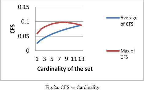
Considerable dip in the value of the maximum CFS with the increase in cardinality is observed in fig 2a

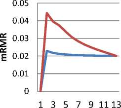
Average of mRMR с    Max of mRMR

Cardinality of the set

Fig.2b. mRMR vs Cardinality

In fig 2b, similarly, average mRMR versus the cardinality of the feature subsets has been plotted. The dip in the cardinality of the feature subset, is much more evident in case of mRMR.

As a next part of the empirical study, we attempt to explore, if the best feature subset in terms of the above metric, results in best classification accuracy?

Both CFS and mRMR have been used to select the best feature subsets and instead of the best feature subset, top three feature subsets based on both the metrics are selected. They have been used to train three different classifiers namely, SVM, Decision tree and naïve Bayes. The results of the same are shown in Table 1. Rank 1, Rank 2 and Rank 3 indicate, the best three feature subsets as per CFS and mRMR.

Table 1. Classification Accuracy of various subsets

	CFS			mRMR
	SVM	Decision Tree	Naïve Bayes	SVM	Decision Tree	Naïve Bayes
Rank 1	88.89	83.33	85.18	77.8	77.78	75.92
Rank 2	85.18	83.3	83.33	75.92	77.8	75.92
Rank 3	90.7	83.33	83.3	75.92	77.8	75.92

The summary of the above study is

• -    Even in a small dataset like wine, no. of subsets is 8191. So an exhaustive search over a medium and large sized dataset for best feature subset will be prohibitively expensive.

• -    The best metric value when grouped by cardinality of the feature subsets seems to be decreasing, with the cardinality of the subsets as demonstrated in fig 2a and fig 2b.

• -    Best three feature subsets are selected and it can be seen, that the best feature set, may not produce the best classification accuracy. As an example, the 3^rd ranked feature subset by CFS when trained with SVM seems to produce a better result than the 1^st Rank and 2^nd Rank. This makes the feature selection problem more appropriate for GA, which can produce multiple near optimal solutions.

• C.    Proposition of our Score (fRMRRP)

The proposed fitness function (fRMRRP) focuses on filtering redundancy, maximizing relevance, and reduced penalization for cardinality of the feature subsets.

Relevance has two components

• -    relevance with the class, measured by mutual information

• -    relevance of the attribute as measured by entropy

For filtering the redundant attributes, Pearson’s correlation coefficient has been used. If the absolute value of the correlation between two variables is greater than a certain threshold then one of them is filtered out. The attribute with higher correlation with the class is retained. Suppose the threshold value is set at 0.8 and feature b and feature c has correlation value of 0.9 and mutual information of the features b and c with the class are 0.5 and 0.6 respectively, then only feature c will be included.

S fRM rrp = (a 'b ... I (fi. ,C) + b* Z_{/ iES} E (f t )) / f (k) )

• -    I(x,y) indicates some numerical measurement of relation between x and y

• -    ‘C’ indicates the class or the target variable

• -    ‘E’ indicates information content in individual

attribute

• -    ‘S’ indicates the selected feature set

• -    ‘k’ is the cardinality of the selected features set

• -    f(k) is a function of k

fRMRRP uses 3 parameters, ‘a’ as a weight for relevance with the class, ‘b’ as a weight for individual relevance and ‘c’ as a threshold value. Both, ‘E’ and ‘I’ are scaled between [0, 1] for better comparison. As explained earlier, absolute value of Pearson correlation coefficient has been used for filtering redundant attributes. Pearson’s correlation coefficient is often criticized because of its linearity and normalcy assumptions. Still it has been chosen because firstly, it’s the most widely used measure and is well understood by research community; secondly it has a very well defined range and associated semantics. The different values that have been used are 0.75 for ’a’, 0.25 for ‘b’ and 0.8 for ‘c’ respectively. For f (k), a sub-linear function is recommended which grows at a lower rate than the linear one. For the experimental setup, square root of k has been used.

• IV.    Experiment Setup

In this section, different steps of the experiment have been detailed. The descriptions of the software tools and libraries as well as the datasets used are enclosed. The parameter values as required by the algorithms and the measures are also discussed.

• i.    The feature sets are represented as binary strings or ‘chromosomes’ as refereed by GA terminology.

• ii.    The different parameters used for GA are :

• i)    0.7 for crossover probability

• ii)    0.05 for mutation probability

• iii)    Population size is taken as 10 * n , where n is the no. of features

• iv)    The maximum iteration count used is 200

• v)    The fitness function used is fRMRRP as described in section III

• iii.    The experiments have been conducted on 21 well known publicly available datasets using a) CFS b) mRMR and c) fRMRRP as the fitness functions. The datasets are quite varied given that some of the datasets have as many as 85 features and 41 labels as enclosed in table 2.

Table 2. Dataset details

Dataset	# Attributes	#Class
Darma	34	6
Hepatatitis	19	2
Seeds	7	3
Glass	9	6
Wine	13	3
Cleaveland	13	5
Breasttissue	9	6
Sonar	60	2
Heart	13	2
Wbdc	30	2
Specftfheart	44	2
Ilpd	10	2
Biodeg	41	2
Optdgt	64	10
Ion	33	2
Pageblocks	10	5
Waveforms	21	3
Veichle	18	4
Bands	19	2
Textue	40	10
Coli	85	41

• iv.    Classification Accuracy (Eqn. 5) have been used for comparing the performance of the methods, Support

Vector Machine (SVM) has been used as the classifier.

The datasets used are listed in table 2, they are taken from public sources [12] and [13] and hence the results are easily reproducible.

‘R’ [15] has been used as the computing environment. Different libraries of ‘R’ namely ‘GA ‘[14], ‘e1071’ [16], ‘entropy’ [23] have been used for the experiment. As the name of the libraries suggest,

• i) . ‘GA’ has been used for genetic algorithm implementation

• ii) . ‘e1071’ has been used for implantation of SVM

• iii) . ‘entropy’ has been used to estimate entropy and mutual information

• v.    In case of multiple feature subsets having same value of the metric, the common features are selected. It was observed that fRMRRP produced more no. of feature subsets as optimal than the other two methods. So if following three feature subsets are tied as best feature subsets as shown in table 3, the feature subset consisting of {F1, F3, F6} is selected. The example assumes a dataset with 6 features namely F1, F2, F3, F4, F5 and F6 respectively.

Table 3. Illustration using fRMRRP

	F 1	F 2	F 3	F 4	F 5	F 6
Feature Subset 1	√		√		√
Feature Subset 2	√					√
Feature Subset 3		√	√			√
Total Presence	2	1	2	0	1	2

• V.    Results and discussion

In this section, the results of the different experiments have been enclosed and critically discussed. In subsection A, the classification accuracy using different methods have been compared and the difference has been tested for statistical significance. In subsection B, the average classification accuracy has been presented with no. of classes in each dataset.

• A.    Analyzing the classififaction accuracy

The classification accuracy with SVM [16] has been presented in table 4. There are other measures of a classifier performance like precision, recall, f-score, ROC etc and classification accuracy is not a good indicator when there is a high class skew. Classifier accuracy is one of the most used metrics to assess performance of a classifier. At first, the classification accuracy, with all features is computed. Three feature subsets are found using GA with a) CFS b) mRMR c) fRMRRP respectively as fitness functions. Classification accuracy is calculated on separate models built on these three feature subsets. Classification accuracy is a ratio given by

# of correctly classified Instances # Instances

The comparison has been given in table 4.

Table 4. Comparison of classification accuracy between all features and that from GA

dataset	All features	CFS	mRMR	fRMRRP
Seeds	95.23	95.23	82.53	90.47
Glass	69.23	46.15	47.69	66.15
Breasttissue	65.62	34.37	37.5	62.5
Ilpd	70.68	70.68	70.68	71.26
Pageblocks	95.24	95.49	91.65	92.65
Wine	100	96.29	83.33	96.29
Cleaveland	62.22	57.78	57.78	61.11
Heart	76.54	70.37	71.6	76.54
Veichle	75.59	35.43	52.75	71.25
Hepa	83.33	83.33	83.33	83.33
Bands	67.27	57.27	59.09	70
Waveforms	86.26	33	33.33	54.26
Wbdc	96.49	85.96	66.08	95.9
Ion	94.33	79.24	73.58	87.73
Darma	95.37	64.5	57.88	93.51
Textue	98.84	98.42	16.05	84.31
Biodeg	87.06	67.82	67.82	86.75
Specftfheart	85.18	86.41	85.18	87.65
Sonar	85.48	73.02	52.38	85.71
Optdgt	65.79	63.66	36.34	98.76
Coli	71.49	74.61	47.09	77.26

Average measure is not very scientific because may be in 5 out of 6 cases method 1 performs better than method2, but in one case method 2 performs better and by a significant margin. The paired t - test can be an option, but it will generate too many combinations. So, as suggested in [17], Friedman’s non-parametric test is employed. Other popular measures like ANOVA could have been used. Friedman test has been given preference because of no assumption about the underlying model.

Given a data [x _i j ] _n*k is to be replaced by [ r _i j ] _n*k where r ij denotes the ranks, in case of a tie , r ij is replaced by an average value of the ranks when a tie occurs. The average rank is given in the equation below.

r.j = ; ∑?=lry                      (6)

The mean ranks, obtained for all the four feature sets is given in table 5.

Table 5. Mean rank of the feature sets

Method	Mean Rank
CFS	2.88
mRMR	3.52
fRMRRP	1.98
All features	1.62

The Friedman statistics has a very low p value with a degree of freedom 3. So the null hypothesis that, there is no difference between the four methods is rejected. As the no. of features increase, fRMRRP seems to perform better, in the 6 datasets which has attributes greater than 40, fRMRRP gives a better mean rank, than with full feature subset. However, this can only be concluded when tested over a large no. of datasets.

One of the important considerations of any feature selection method is that the performance achieved using reduced feature subset and the performance achieved using all features should be equivalent or close. A paired t-test have been conducted between classification accuracy achieved by the following three paired combinations.

• a)    Selected feature sets through CFS (S CFS ) and all features

• b)    Selected feature sets through mRMR (S mRMR ) and all features

• c)    Selected feature sets through fRMRRP (S fRMRRP ) and all features

The p-values of the above comparisons are enclosed in Table 6a.

Table 6a. Paired t-test results all features and the three methods

Comparison	p-value
All and S CFS	0.001
All and S mRMR	0.00007
All and S fRMRRP	0.09

So it can be observed that the null hypothesis for the first two cases can be rejected, but the null hypothesis for the third case cannot be rejected. Thus it can’t be concluded that the difference between results obtained with all features and S mRMRFP is statistically significant. However, the difference in results using the full feature set as compared to using CFS and mRMR is not due to chance at a critical value of even 0.01.

A comparison as presented in table 6b, also have been done between mRMRFP , CFS and mRMR for statistical significance of the difference.

Table 6b. Paired t-test results between fRMRRP and other two methods

Comparison	p-value
S fRMRRP and S CFS	0.003
S fRMRRP and S mRMR	0.00004

From the above table, the null hypothesis that there is no no statistically significant difference is rejected. The overall reduction in feature sets is 39.5% and on the average it is 37.63% by the proposed method. It is to be noted, the average reduction in no. of features in case of fRMRRP is lesser than CFS or mRMR. mRMR has the highest reduction rate , but at the same time the worst classification accuracy.

• B.    Average classififaction accuracy and .no of classes

As the no. of classes or labels increases in a dataset, the harder the problem becomes. In table 7, the datasets have been grouped by the .no of classes they have.

Table 7. Average Classification accuracy by # Classes

#Class	All features	CFS	mRMR	fRMRRP
2	82.9	74.9	70.0	82.8
3	93.8	74.8	66.4	80.3
4	75.6	35.4	52.8	71.3
5	78.7	76.6	74.7	76.9
6	76.7	48.3	47.7	74.1
10	82.3	81.0	26.2	91.5
41	71.5	74.6	47.1	77.3

The above table is also represented using a line graph , to appreciate the relation between average classification accuracy and no. of classes. The comparison has been shown between”all features” and “selected features” by proposed method.

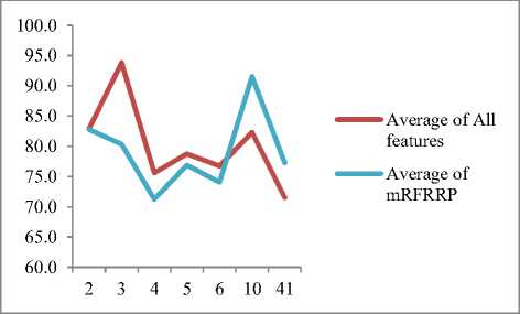
Fig.3. Comparing average classification accuracy by # of classes.

It is observed that , the average classification accuracy using the porposed method becomes better , as the no. of classes increase.

• VI. Conclusion

In this paper, a novel measure (fRMRRP) for feature subset quality has been proposed which refines the notion of relevance and redundancy of a feature. This has been used as fitness function i.e. an optimization objective for Genetic Algorithm. The proposed method achieves close to 40% reduction in cardinality of feature set. When compared with all the features, the said reduction is achieved without any statistically significant performance degradation measured in terms of classification accuracy. The proposed metric seem to deliver superior results as the no. of classes or labels and size of the dataset increase. It produces better performance compared to feature subsets selected using CFS and mRMR and the gain in performance is statistically significant. The results also indicate potential of superior performance even compared with all features for high dimensional feature set. As an extension of the work, a study on tuning the various parameters of fRMRRP and experiments with larger datasets is planned.