A Simple Statistical Model to Estimate Incident Solar Radiation at the Surface from NOAA AVHRR Satellite Data

Published Online January 2013 in MECS

The data of solar radiant energy incident on the earth’s surface and its distribution is gaining increasing importance, not only in solar energy development but also for agriculture, weather and climate monitoring and predictions. Solar radiation falling on the earth’s surface in the visible and near-infrared wavelength range (0.3μm – 3.0μm) is usually measured on the ground by means of pyranometers. But this needs hundreds of pyranometer stations to map the spatial variability of solar irradiance for a larger region. This is practically impossible, because ground measurements suffer from high costs for purchasing of equipment, adequate maintenance and time consuming data screening. An alternate solution to this problem is to calculate the distribution of solar radiation incident on the earth through the analysis of images of meteorological satellites. Thus, proper processing of satellite data provides a wealth of information needed in the production of solar atlases which is useful for planning purposes [1],[2].

In this work we have developed a model to estimate hourly solar radiation incident on the earth’s surface by analyzing digital images of National Oceanic and Atmospheric Administration (NOAA) of USA polar orbiter satellite. When crossing the atmosphere, solar radiation suffers complex interactions of scattering and absorption by the atmospheric components. The degree of these interactions varies considerably from place to place and season to season. Also, the complex geometry between the sun, satellite and earth makes the satellite based solar radiation estimation a time consuming and relatively difficult task. In our method, we have used statistical regression technique which requires ground measured data as the input for the satellite based methodology [3],[4],[5].

The basic idea of this method is that the amount of the cloud cover over a given area statistically determines the global radiation for that area. Thus the processing is divided into two steps: a cloud cover index (presence of cloud and its optical property) is derived for each location or pixel of the original satellite image and subsequently used in a second step for a statistical estimation of the global radiation [6].

One of the most important factors that affect both the incoming solar radiation at the earth’s surface and the solar radiation emerging from the atmosphere, is the change in the sun zenith angle and the corresponding change in the air mass through which the sun radiation travels.

The second largest cause results from the presence of clouds. The presence of water droplets and of ice particles in clouds strongly increases both the absorption and scattering of solar radiation.

The goal of the work is to show the entrance and overview methodology of the satellite monitoring of the earth by remote sensing. Many algorithms have been developed for its estimation from satellite data. In a review paper, Noia et al. (1993) described the best known methods developed using both the statistical and physical models from geostationary satellite data. Also there are some other methods developed from sun synchronous polar orbiter satellite data [7], [8].

The remainder of this paper organized as follows. Section II provides the operational procedure of determination of the cloud cover index, relation between cloud cover index and ground measured transmission factor, and determination of hourly global radiation at ground. Section III explains the results and discussion from the training data set and estimation data set. Conclusion is given in the final section.

• II.    Operational Procedure

• 2.1    Determination of Cloud Cover Index^[9]

• 2.2    Statistical relationship between Cloud Cover Index and Ground Measured Transmission Factor ^[9]

The method used in this study is a statistical one. In this method, satellite images are processed as monthly basis. Each pixel of one image has been compared to the corresponding pixels of all images of the given month and the minimum values obtained for each pixel has been retained. The image thus obtained is called reference ground albedo image. The same procedure has been followed taking the maximum values for each pixel for the same time series images of the month and has been retained as reference cloud albedo image.

In this work, the study area is the geographical area at Bogra in Bangladesh which is located between 24 ° 85 ‘ north latitude and 89 ° 37 ‘ east longitude.

The cloud cover index n^t(i, j) at point (i, j) for a given time t is defined as a function of the ground reference albedo p(i,j) , the instantaneous albedo at the same point as measured by the satellite p (i, j) and the cloud reference albedo p c .

It is computed for each pixel using the following formula nt(i,j) = [p(i,j) - P(iJ)] / [pc - p(i, j)]              (1)

The magnitudes of cloud cover index ranges from 0 to 1 and can be interpreted as the percentage of the cloud cover per pixel.

The method uses linear regression between the satellite determined cloud cover index and the ground measured transmission coefficient. This simple and efficient approach is based on previous work from Bourges.

The total atmospheric transmission factor K(i, j) is defined as the ratio of global radiation at ground on a horizontal surface G(i, j) to the irradiance outside the atmosphere G 0 (i, j)

K(i, j) = G(i, j) /G 0 (i, j)                                 (2)

This quality ranges from 0.2 to 0.8. if one interprets the cloud cover index nt(i , j) as the percentage of pixel covered by clouds, the global ground irradiance at time t is expressed as a linear combination

G(i, j) = n^t(i, j) G b (i, j) + (1- n^t(i, j)) G c (i, j)      (3)

Where,

G b is the global ground irradiance for overcast

G_c is the global ground irradiance for clear skies.

For each of these extreme condition, one can define a transmission factor respectively K b and K c which is supposed to be constant for a given hour. This realistic hypothesis leads to the following linear relation

K^t(i , j) = n^t(i, j)K b (i, j) + (1- n^t(i, j))K c (i, j)

= n^t(i, j)(K b (i, j) - K c (i, j)) + K c (i, j)

= a(i, j) n^t(i, j) + b(i, j)                         (4)

Where coefficient a corresponds to the slope of the curve and b represents the atmospheric transmission factor with a clear sky, which is a more stable coefficient than a , which is extremely influenced by cloudiness conditions. The a and b are assumed to be constant for a period of one month for each point of the surface.

• 2.3    Determination of Hourly Global Radiation at Ground

If it is assumed that the field of coefficients a and b for each pixel is stable in time or slowly varying on a seasonal basis. It is thus possible to estimate the transmission factor for each new image as follows

K^t(i, j) = a(i, j) n^t(i, j) + b(i, j)                          (5)

The estimation of the hourly global radiation is then deduced as follows

G h (i, j) = K^t(i, j) G 0 (i, j)                                   (6)

For satellite images, the procedure consists of working with a set of images, in this case, all dynamic images of the months; May and November. The visible image channels are used to detect the clouds and the albedo of both the ground and the clouds. The cloud cover index is determined by applying a statistical procedure. The images for the months under analysis are taken and the minimum value for each pixel is taken that give the information of the cloud reference albedo and ground reference albedo. Then the cloud index is determined for each pixel by application of equation(3).

Coefficients a and b are determined from field data defining a linear regression between a transmission factor deduced from the solar radiation data measured at ground and the cloud index at the same location determined from satellite. Hourly global solar radiation was then determined for the whole study area using the procedure shown in Fig. 1. [9]

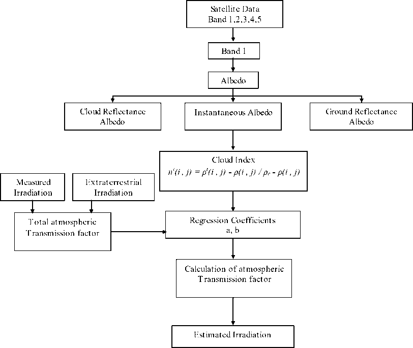
Fig. 1: Image Processing Diagram

Table 1: Training dataset of Bogra. May

Date	Extraterrestrial Irradiation	Measured Irradiation	Cloud Index	Total Atmospheric Transmittance Factor
3	1251.48	786	0.007	0.6280551
4	1193.59	476	0.185	0.3987985
5	1170.52	200	0.785	0.1708639
7	1259.44	432	0.428	0.3430105
11	1273.86	853	0.008	0.6696208
12	1273.86	683	0.309	0.5361677
15	1286.27	565	0.236	0.4392562
16	1251.48	727	0.1	0.580911
18	1158.31	252	0.57	0.2175586
20	1280.31	163	0.997	0.1273126
21	1243.04	452	0.163	0.3636255
23	1308.36	783	0.088	0.5984599
27	1170.52	574	0.153	0.4903794
29	1273.86	487	0.24	0.382304
30	1234.1	945	0.049	0.7657378
31	1182.28	355	0.36	0.3002665

• III.    Results and Discussion

The data from satellite sensor provides information about the presence and its optical properties of clouds. On the other hand, data from ground measurements provide information about the atmospheric transmissivity. In our method, the monthly data set (cloud index and atmospheric transmission factor) are divided into two groups by random choice. One group is called ‘training data set’ shown in Table 1 and Table 3. On the other hand, the other group is called ‘estimation data set’ shown in Table 2 and Table 4. From the training data set regression coefficients ‘a’ and ‘b’ are obtained from the linear relation of Equation (6). Here the coefficient ‘a’ represents the slope and ‘b’ represents the intercept of the line. These coefficients are then applied on the estimation data set to determine the hourly incident radiation on the earth’s surface.

Table 2: Estimated Dataset for Bogra, May

Date	Extraterrestrial Irradiation	Total Atmospheric Transmittance Factor	Calculated Atmospheric Transmittance Factor	Regression Coefficient		Cloud index	Estimated Irradiation	Measured Irradiation Wh m-2
				a	b
1	1132.55	0.4821	0.4625	-0.5724	0.6056	0.25	523.802	546
9	1259.44	0.56374	0.5672492	-0.5724	0.6056	0.067	714.414	710
17	1214.79	0.11525	0.2186576	-0.5724	0.6056	0.676	265.624	140
28	1296.64	0.4396	0.545498	-0.5724	0.6056	0.105	707.316	570

Table 3: Training dataset of Bogra, November

Date	Extraterrestrial Irradiation	Measured Irradiation	Cloud Index	Total Atmospheric Transmittance Factor
2	1280.313	614	0.087	0.47957027
6	1291.71	708	0.051	0.54811075
8	1214.793	509	0.319	0.41900156
9	1170.522	403	0.392	0.34429078
10	1316.714	561	0.123	0.42606048
13	1193.585	641	0.099	0.53703748
14	1304.97	538	0.11	0.41227009
15	1280.313	508	0.108	0.396778
20	1204.423	151	0.97	0.12537119
22	1170.522	447	0.145	0.38188084
23	1301.064	438	0.404	0.3366475
24	1273.855	357	0.352	0.28025163
27	1304.97	601	0.042	0.46054707

Table 4: Estimated Dataset for Bogra, November

Date	Extraterrestrial Irradiation	Total Atmospheric Transmittance Factor	Calculated Atmospheric Transmittance Factor	Regression Coefficient		Cloud index	Estimated Irradiation	Measured Irradiation Wh m-2
				a	b
7	1259.437	0.5145	0.4895584	-0.3927	0.493	0.008	616.5678	648
12	1234.104	0.3622	0.4353658	-0.3927	0.493	0.146	537.2867	447
21	1224.688	0.3772	0.3862783	-0.3927	0.493	0.271	473.0703	462
26	1291.71	0.3731	0.359182	-0.3927	0.493	0.34	463.9589	482

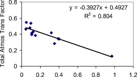
Data of two months (May and November) have been processed for this work. Fig. 2 and Fig. 3 give the graph for finding regression coefficients ‘a’ and ‘b’ for all the months for ground measurement points. The regression equation and correlation of coefficient (R squared values) are also shown.

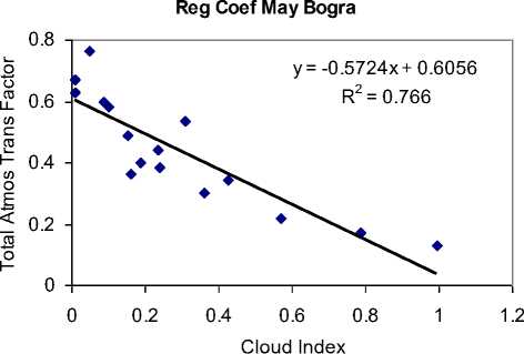
Fig. 2: Linear regression between the total atmospheric transmission factor and Cloud index for Bogra, May

Reg Coef Nov Bogra

Cloud Index

Fig. 3: Linear regression between the total atmospheric transmission factor and Cloud index for Bogra, November

Performance of the method in estimating global solar radiation has been tested by calculating relative deviation, denoted by d, between the estimated and measured values. Table 5 and Table 6 present the relative deviation for all the data points for the study period. For few points it goes high. This result indicates that the method can be used for estimation of solar radiation on the surface of Bangladesh.

Table 5: Relative Deviation for Bogra, May

Date	Estimated Irradiation	Measured Irradiation	Relative Deviation, d
1	523.802	546	-0.04
9	714.414	710	0.006
17	265.624	140	0.89
28	707.316	570	0.24

Table 6: Relative Deviation for Bogra, November
Date	Estimated Irradiation	Measured Irradiation	Relative Deviation, d
7	616.5678	648	-0.04
12	537.2867	447	-0.2
21	473.0703	462	-0.02
26	463.9589	482	-0.03

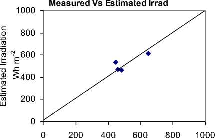
Using the regression coefficient values, solar radiation incident on the earth surface has been determined using the above equations. Fig 4 and Fig 5 gives the scatter plot between pyranometer measured and satellite estimated irradiation values for the study period. In these scatter plots, the diagonal line shows the exact fit between the measured and estimated values.

Measured Vs Estimated Irrad

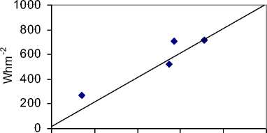
0    200   400   600   800  1000

Measured Irradiation Whm-2

Fig. 4: Comparison Between satellite-estimated and Pyranometer-measured hourly global solar radiation for Bogra, May

Measured Irradiation Wh m-2

Fig. 5: Comparison Between satellite-estimated and Pyranometer-measured hourly global solar radiation for Bogra, November

• IV.    Conclusion

In this paper, a simple statistical method has been presented for retrieval of incident solar radiation from a polar orbiter satellite data. The accuracy of the method has been tested by calculating relative deviation between the ground measured and satellite estimated values. The results thus obtained have been compared with other methods. It is found that the method’s output has reasonably good agreement between the measured and model estimated radiation values.