Accelerating Activation Function for 3-Satisfiability Logic Programming

Author: Mohd Asyraf Mansor, Saratha Sathasivam
Journal: International Journal of Intelligent Systems and Applications(IJISA) @ijisa
Article in issue: 10 vol.8, 2016.
Free access
This paper presents the technique for accelerating 3-Satisfiability (3-SAT) logic programming in Hopfield neural network. The core impetus for this work is to integrate activation function for doing 3-SAT logic programming in Hopfield neural network as a single hybrid network. In logic programming, the activation function can be used as a dynamic post optimization paradigm to transform the activation level of a unit (neuron) into an output signal. In this paper, we proposed Hyperbolic tangent activation function and Elliot symmetric activation function. Next, we compare the performance of proposed activation functions with a conventional function, namely McCulloch-Pitts function. In this study, we evaluate the performances between these functions through computer simulations. Microsoft Visual C++ 2013 was used as a platform for training, validating and testing of the network. We restrict our analysis to 3-Satisfiability (3-SAT) clauses. Moreover, evaluations are made between these activation functions to see the robustness via aspects of global solutions, global Hamming distance, and CPU time.
3-Satisfiability, Hyperbolic tangent activation function, Elliot symmetric activation function, McCulloch-Pitts function, Logic programming, Hopfield neural network
Short address: https://sciup.org/15010865
IDR: 15010865
Text of the scientific article Accelerating Activation Function for 3-Satisfiability Logic Programming
Published Online October 2016 in MECS
Artificial intelligence is one of the most eminent and staple fields in mathematics, physics, and computer science [2]. In fact, the emergence of artificial intelligence attracted a prolific amount of research in combinatorial optimization problems [3, 8]. In addition, the popularity of artificial intelligence is due to the ability to solve many computational, classification, and pattern recognition problems via learning based algorithm [7, 21]. Generally, the integration of neural network, logic programming, and satisfiability problem are vital in enhancing the artificial intelligence field. As we all know, there are numerous neural networks, from the modest to intricate, similarly to the evolution human biological nervous system [5]. The popularity of artificial neural network is due to the collective behavior of the network, inspired by the biological human brain. Thus, the network can be hybridized with some other computational methods in order to solve sophisticated problems and applications.
One of the well-known neural networks is Hopfield neural network. Specifically, the Hopfield network is a recurrent neural network introduced by John Hopfield [3]. It is renowned for the remarkable power in learning, memory and storage [1, 11, 18]. The Hopfield model is a conventional model for content addressable memory (CAM) [1, 8]. It is an important feature of Hopfield which motivated by the manner of biological brain works. In addition, Hopfield network comprised of a set of N interconnected neurons which all neurons are connected to all others in both directions [6, 13]. Then, the Hopfield neural network can be demarcated as a simple recurrent network which can work as an efficient associative memory, and it can store definite memories [1, 2]. One of the popular work is done by Little who proposed a little Hopfield network based on the energy minimization scheme. Moving on, Sathasivam introduced a powerful Hopfield model based on reverse analysis method in solving Horn-satisfiability problem [14, 22]. The work on Hopfield network is still ongoing for the promising future work. Moreover, the Hopfield model is a branch of neural network that been applied in various mathematical problems such as Travelling Salesperson problem (TSP), scheduling, pattern recognition, and satisfiability problem.
This paper is organized as follows. Part II introduces the fundamental concept of 3-Satisfiability and logic programming. In section III, the Hopfield neural network is discussed briefly. Besides, section IV covers conceptual discussion of activation functions. In section V, theory implementation of the activation functions is been discussed. Finally, section VI and VII enclose the experimental results and conclusion of this research.
-
II. 3-S ATISFIABILITY P ROBLEM
Strictly speaking, satisfiability (SAT) can be defined as the task of searching a truth assignments that creates an arbitrary Boolean expression true [4, 7]. Basically, the satisfiability problem can be treated as the combinatorial optimization problem according to logic programming perspective. In other words, satisfiability problem refers to decision making problems based on particular constraints. On the contrary, k-SAT problem is deliberated as a NP problem or non-deterministic problem.
The three core components of k-SAT are summarized as follows:
logical operator OR. Each clause must consist of k variables.
In this paper, we only focus on 3-Satisfiability (3-SAT) clauses.
-
A. 3-Satisfiability Problem
In this paper, we emphasize a paradigmatic NP-complete problem namely 3-Satsifiability (3-SAT). Generally speaking, 3-SAT can be defined as a formula in conjunctive normal form where each clause is limited to at most or strictly three literals [16]. The problem is an example of non-deterministic problem [15]. In our analysis, the following 3-SAT logic program which consists of 3 clauses and 3 literals will be used. For instance:
P =( AvBvC )л( AvBvC )л( AvBvD ) (1)
We represent the above 3 CNF (Conjunctive Normal Form) formula with P. Thus, the formula can be in any combination as the number of atoms can be varied except for the literals that are strictly equal to 3 [19]. Hence, it is vital for combinatorial optimization problem. The higher number of literal in each clause will increase the possibilities or chances for a clause to be satisfied [17].
The general formula of 3-SAT for conjunctive normal form (CNF):
P = A , = 1 Z i (2)
So, the value of k denotes the number of satisfiability [21]. In our case, k-SAT is 3-SAT.
k
Zi=Aj=i(ХУ,Уу,zj),k > 3 (3)
-
B. 3-SAT Logic Programming
Logic programming is the integration of mathematical logic and neural network concept [21]. Logic is deals with true and false while in the logic programming, a set of clauses that formed by atoms are represented to find the truth values of the atoms in the clauses [7, 14]. We use neurons to store the truth value of atoms to write a cost function for minimization when all the clauses are satisfied [6]. The reason we implement logic programming is as follows:
-
i) Logic program is writable and readable.
-
ii) Well-founded semantic for further simplification.
-
iii) Flexible and easy to implement with the other algorithm.
-
iv) Can be treated as a problem in combinatorial optimization.
So, we can set the Boolean formula according to the clauses that we want. Hence, we can easily integrate the
3-SAT logic programming with Hopfield neural network.
Based on Sathasivam’s method [1, 14], the following algorithms summarize on 3-SAT logic programming in Hopfield network.
-
i) Given a logic program, translate and transform all the 3-SAT clauses in the logic program into basic Boolean algebraic form.
-
ii) Recognize a neuron to each ground neuron according to the 3-SAT principles.
-
iii) All connections strengths are initialized to zero. Hence, it assumed the connection with A, B and C is zero value. The other connection strengths are computed by implementing the cost function and Hopfield energy function.
-
iv) Derive a cost function that is incorporated with the negation of all clauses. For example, X = 1 ( 1 + Sx ) and X = 1 ( 1 - Sx ) . Sx = 1 (True)
and S X = - 1 (False). Multiplication represents CNF and addition represents DNF.
-
v) Comparing the cost function with energy by obtaining the values of connecting strengths. The values of the connection strengths or weights are vital in logic programming.
-
vi) Let the neural network to progress until minimum energy is reached. The neural states then provide a solution interpretation for the logic program.
-
vii) Next, verify whether the solution obtained is a global solution or not.
viii) Compute the global minima ratio, Hamming distance and CPU time.
-
III. D ISCRETE H OPFIELD N ETWORK
Discrete Hopfield neural network is staple in numerous aspects in artificial intelligence and logic. As an expended form of Hopfield network illustration, discrete Hopfield network is the simplest form [1]. Generally, Hopfield network is extensively been used to solve combinatorial optimization problem and content addressable memory. Beside, Hopfield network has few remarkable features.
One of the features is distributed representation [18]. Hence, memory can be stored as a pattern and overlay upon one another different memories over the equivalent set of processing elements [2, 14]. Order than that, it is distributed and asynchronous control. Every single processing agent creates their own decisions according to their local circumstances [4, 5]. The Hopfield neural network is an attractor neural network. Thus, the units in Hopfield nets are called binary threshold unit [1], which strictly take binary values such as 1 and -1. The fundamental delineations for unit I’s activation, ai are given:
ai
' 1 if £ wy8j > ^
- 1 Otherwise
Where w ij is the connection strength from unit j to i .
We focus on Hopfield energy minimization function in solving combinatorial optimization or satisfiability problem [6]. Hence, an energy function for the discrete Hopfield networks for second order Hopfield networks is formulated as follows:
h i = E j S j + w" (5)
Since the Lyapunov function is decreasing monotonically with the dynamics. The two-connection model can be generalized to include higher order connections. The “local field” equation is simplified into hi
• •+EEww + Em+ w I j k j
Where “…..” indicates still higher orders, and an energy minimization function can be written as follows:
E=••- 1 ZZEwijkxixjxk- 1 EZwjxXj- Ewi-xi
3i jk 2i ji provided that Jijk = J[ijk] for i, j, k distinct, with […] denoting permutations in cyclic order, and Jijk = 0 for any i, j, k equal, and that similar symmetry requirements are satisfied for higher order connections.
The updating rule maintains as in (8).
S i ( t + 1 ) = sgn [ h i ( t ) ] (8)
The network is set up in an initial state, released, and the dynamics will take the network to the closest fixed point. The job of the learning rule of a Hopfield network is to find some weight matrix which stores the required patterns as fixed points of the network dynamics so that patterns can be recalled from noisy or incomplete initial inputs.
The relaxation technique in Hopfield network is an essential method for using contextual information to minimize local uncertainty and achieve global consistency in many applications [2]. Haykin highlighted the solution of an optimization problem for Hopfield neural network can be obtained systematically after the network undergoing relaxation process [5]. Since we are treating the 3-SAT problem as an optimization problem, Sathasivam’s relaxation technique can be employed in order to guarantee the network relaxed to the equilibrium state [14].
Precisely, this technique will control certain parameter in the energy function. The function of the relaxation rate in the network dynamics is to regulate the rapidity of the relaxation so that solutions with superior quality can be achieved. According to Sathasivam [1, 14], the network will undergo the relaxation process in order to increase the convergence of the solutions. Thus, the input of the neuron is reorganized via the following equation:
dhi new dhi
= R dt dt (9)
r represents the relaxation rate and h denotes to the local field as in equation (6).
Hence, if output exceeds the threshold value, the actual state is 1 else the value of the actual state is -1. The updated neuron states via activation functions are crucial in hunting the optimal state which may lead to global solutions. We will implement the following formula after performing the computation in equation (6), (7) and (8).
-
A. McCulloch-Pitts Function/Linear Activation Function
The McCulloch-Pitts model of a neuron is simple yet has considerable computing prospective. The McCulloch-Pitts function is also has precise mathematical definition and easy to implement. However, this model is so simplistic and tends to generate local minima outputs [9, 14]. Many researcher urged the alternatives for this function as it is very primitive and leads to slower convergence.
-
IV. P OST O PTIMIZATION T ECHNIQUE : A CTIVATION F UNCTION
According to [14], the solutions of McCulloch-Pitts function will stuck easily in local minima of the energy and it is time consuming to achieve global solutions. Hence, it doesn’t reduce the computation burden for training the network.
In our analysis, we integrate the Hyperbolic tangent activation function and Elliot symmetric activation function as catalyst for 3-SAT logic programming in Hopfield network. We combine the advantages of each activation function and Hopfield neural network as a single hybrid network. Other than that, activation functions will be tested as a medium to check the network complexity.
Strictly speaking, the activation function are commonly used to transform the activation level of a unit (neuron) into an output signal in neural network [8]. In layman’s term, it is also known as transfer function or squashing function due to the capability to squash the permissible amplitude range of output signal to some finite value [9].
In our study, we punch in the value obtained from the local field equation into the value of x for each of our activation. Hence, the Hopfield local field value is vital before squashing it into the activation function as the input [8, 22]. Then, the formula of generating the output can be summarized as follows:
y ( x )
I- 1, g ( x i ) < 0
1+ 1, g ( x i ) ^ 0
g( X ) = X (11)
Another drawback is the linear activation function will only produce positive numbers over the whole real number. Thus, the output values are unbounded and not monotonic. Hence, the outputs obtained will diverges from the global solutions.
-
B. Hyperbolic Tangent Activation Function
Hyperbolic tangent activation function is proven as the most powerful activation function in neural network. Hence, we want to investigate whether the robustness of this function will apply to the 3-SAT logic programming. Generally, this function can be defined as the ratio between the hyperbolic sine and the cosine functions expanded as the ratio of half-difference and half-sum of two exponential functions in the points x and –x [8, 14].
The main feature of Hyperbolic tangent activation function is the broader output space than the linear activation function. The output range is -1 to 1, similar to the conventional sigmoid function. The scaled output or bounded properties will assist the network to produce good outputs. Hence, the outputs will converge to the global solutions. The hyperbolic tangent activation function can be visualized as follows:
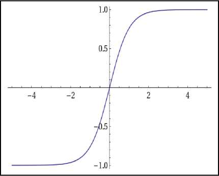
Fig.1. Hyperbolic tangent activation function.
The Hyperbolic tangent activation function is written as follows:
g ( x ) = tanh( x ) = ^inh- x = e x e _ x (12)
cosh( x ) e x + e x
The main feature of Hyperbolic tangent activation function is the broader output space than the linear activation function. The output range is -1 to 1, similar to the conventional sigmoid function. The scaled output or bounded properties will assist the network to produce good outputs. Hence, the outputs will converge to the global solutions.
-
C. Elliot Symmetric Activation Function
According to Sibi et al. [9], the Elliot symmetric activation function is a class of transfer function with higher speed approximation. This activation function has an ability to compute on modest computing hardware as it does not involve any exponential or trigonometric functions. The drawback is that it only flattens out for large inputs, so a small number of outputs produced will be trapped into the local minima. As a result, this might result in more training iterations, or require more neurons to achieve the same accuracy.
g( x ) = X (13)
-
1 + 1 x
The output range for Elliot symmetric activation function is -1 to 1. The performance analysis of Elliot symmetric activation function will be compared with the other counterparts as mentioned earlier.
-
V. I MPLEMENTATION
The implementation consists of methodical procedures. First of all, we define the number of neurons. Next, program clauses are generated randomly based on 3SAT or 1-SAT formula. Thirdly, the initial states are being initialized for the neurons in the clauses.
Then, initialize the connection weights to zero including energy parameters plus with other related parameters for clauses together. The network evolves or relaxes until minimum energy is reached.
During the energy relaxation phase, the neuron state is updated by using activation function. After the network relaxed to an equilibrium state, test the final state obtained for the relaxed neuron whether it is a stable state. If the states remain unchanged for five time steps, then consider it as stable state. Subsequently, compute the corresponding final energy for the stable state. If the difference between the final energy and the global minimum energy is within the tolerance value, then consider the solution as global solution.
Otherwise, we need to return to beginning procedure. Then, we compute the ratio of global solutions and the hamming distance between stable state and global solution. Global solution is the interpretation used in the model for the given logic program or better known as global minima ratio. Global minima ratios are computed via the following formula:
Global Minima Ratio =
Global solutions
Number of iterations
In addition, we run the relaxation for 1000 iterations and 100 combinations to minimize the statistical error. The selected termination criterion is 0.001. Furthermore, all these values are obtained by trial and error technique, where we tried several values as tolerance values and selected the value which yields better performance than other values. Finally, we compared the experimental results such as global minima ratio, Hamming distance and computation time between the McCulloch-Pitts function, Elliot symmetric activation function and Hyperbolic activation function.
-
A. CPU Time
In this paper, the CPU time can be defined as the total time taken for which our network was used for training and generating the maximum satisfied clauses [7, 14]. Hence, the CPU time can be seen as the indicator of the performance of the post optimization paradigms that used in this study.
Table 1. CPU time for various activation functions
|
Number of Neurons |
CPU Time (second) |
||
|
Elliot Symmetric |
McCulloch-Pitts |
Hyperbolic Tangent |
|
|
10 |
4 |
10 |
1 |
|
20 |
25 |
77 |
18 |
|
30 |
80 |
469 |
56 |
|
40 |
222 |
9800 |
156 |
|
50 |
561 |
84356 |
360 |
|
60 |
1230 |
- |
974 |
|
70 |
1888 |
- |
1489 |
|
80 |
5764 |
- |
5002 |
From the table 1, it had shown the CPU time was increased as the network complexity also increased. When we integrate the Hyperbolic tangent activation function in logic programming, this problem can be minimized. So, the Hyperbolic tangent activation function had accelerated the training or computation process in order to obtain global solutions. Hence, the CPU time is faster than the other counterparts due to less computation burden. Hence, less energy is needed to achieve the convergence. From table 1, it can be seen that McCulloch-Pitts function took more time to generate the global solutions for 3-SAT logic programming. The Elliot symmetric activation function recorded good CPU time but still slower than Hyperbolic tangent activation function. Faster computation time is vital in logic programming, as it is an indicator that we can satisfy the 3-Satisfiability problem within the stipulated time-scale.
-
B. The global minima ratio
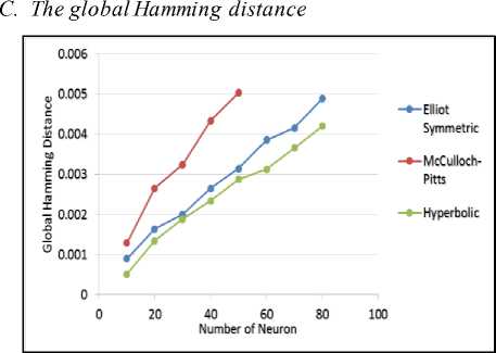
Fig.2. The global Hamming distance in various methods
Table 2. The global minima ratio in various methods
|
Number of Neurons |
Global Minima Ratio |
||
|
Elliot Symmetric |
McCulloch-Pitts |
HyperboliTan gent |
|
|
10 |
0.9981 |
0.9895 |
0.9999 |
|
20 |
0.9902 |
0.9811 |
0.9945 |
|
30 |
0.9843 |
0.9748 |
0.9898 |
|
40 |
0.9796 |
0.9674 |
0.9812 |
|
50 |
0.9710 |
0.9566 |
0.9741 |
|
60 |
0.9656 |
- |
0.9703 |
|
70 |
0.9603 |
- |
0.9658 |
|
80 |
0.9585 |
- |
0.9594 |
Table 2 depicts the global minima ratio obtained from the computer simulation for different types of activation functions. In our analysis, the global minima ratio obtained for the Hyperbolic tangent activation function in 3-SAT logic programming is better than the Elliot symmetric function and McCulloch-Pitts function. According to the global minima ratio achieved for the Hyperbolic tangent activation function, it can be seen that the value is much closer to 1 compared with the Elliot symmetric activation function and McCulloch-Pitts function although we enriched the network complexity by increasing the number of neurons (NN). This is because the Hyperbolic tangent activation function enhanced the energy relaxation process in order to get better solutions. Thus, the global solutions can be obtained perfectly without being stuck in local minima or sub-optimal solutions. This is due to fewer barriers for the neurons to achieve the global solutions. For the 3-satisfiability problem, the McCulloch-Pitts function unable to sustain more neurons due to the complexity. The solutions seem to oscillate and stuck much easier in local minima. For 3-SAT, the McCulloch-Pitts functions only endured and sustained until 50 neurons. The implementation of Elliot symmetric activation function can help to sustain more neurons but the solutions obtained were slightly closer to the Hyperbolic tangent activation function for both satisfiability problem. However, Hyperbolic tangent activation function performs better in generating better global solutions. For instance, the effective updating ability of the proposed model is a key to perform well in 3-satisfiability logic programming.
-
VII. C ONCLUSION
References Accelerating Activation Function for 3-Satisfiability Logic Programming
- S. Sathasivam, P. F. Ng, and N. Hamadneh, Developing agent based modelling for reverse analysis method, Journal of Applied Sciences, Engineering and Technology 6 (2013) 4281-4288.
- R. Rojas, Neural Networks: A Systematic Introduction, Berlin: Springer, 1996.
- J. J. Hopfield and D. W. Tank, Neural computation of decisions in optimization problems, Biological Cybernatics 52 (1985) 141-151.
- U. Aiman and N. Asrar, Genetic algorithm based solution to SAT-3 problem, Journal of Computer Sciences and Applications 3 (2015) 33-39.
- S. Haykin, Neural Networks: A Comprehensive Foundation, New York: Macmillan College Publishing, 1999.
- G. Pinkas, and R. Dechter, Improving energy connectionist energy minimization, Journal of Artificial Intelligence Research 3 (1995) 223-237.
- W. A. T. Wan Abdullah, The logic of neural networks. Physics Letters A 176 (1993) 202-206.
- K. Bekir and A. O. Vehbi, Performance analysis of various activation functions in generalized MLP architectures of neural network. International Journal of Artificial Intelligence and Expert Systems 1(4) (2010) 111-122.
- P. Sibi, S. A. Jones and P. Siddarth, Analysis of different activation functions using back propagation neural networks. Journal of Theoretical and Applied Information Technology 47 (2013) 1264-1268.
- R. A. Kowalski, Logic for problem solving, New York: Elsevier Science Publishing Co, 1979.
- Y. L. Xou and T. C. Bao, Novel global stability criteria for high-order Hopfield-type neural networks with time-varying delays, Journal of Mathematical Analysis and Applications 330 (2007) 144-15.
- N. Siddique and H. Adeli, Computational Intelligence Synergies of Fuzzy Logic, Neural Network and Evolutionary Computing, United Kingdom: John Wiley and Sons, 2013.
- B. Sebastian, H. Pascal and H. Steffen, Connectionist model generation: A first-order approach, Neurocomputing 71(13) (2008) 2420-2432.
- S. Sathasivam, Upgrading Logic Programming in Hopfield Network, Sains Malaysiana, 39 (2010) 115-118.
- B. Tobias and K. Walter, An improved deterministic local search algorithm for 3-SAT, Theoretical Computer Science 329 (2004) 303-313.
- D. Vilhelm, J. Peter and W. Magnus, Counting models for 2SAT and 3SAT formulae, Theoretical Computer Science, 332 (2005) 265-291.
- L. J. James, A neural network approach to the 3-Satisfiability problem, Journal of Parallel and Distributed Computing 6(2) (1989) 435-449.
- H. Asgari, Y. S. Kavian, and A. Mahani, A Systolic Architecture for Hopfield Neural Networks. Procedia Technology, 17 (2014) 736-741.
- P. Steven, SAT problems with chains of dependent variables, Discrete Applied Mathematics 130(2) (2003) 329-22.
- K. Ernst, B. Tatiana and C. W. Donald, Neural Networks and Micromechanics, New York: Springer Science & Business Media, 2009.
- C. Rene and L. Daniel, Mathematical Logic: Propositional Calculus, Boolean Algebras, Predicate Calculus, United Kingdom: Oxford University Press, 2000.
- M. Kaushik. Comparative analysis of exhaustive search algorithm with ARPS algorithm for motion estimation. International Journal of Applied Information Systems 1(6) (2012) 16-19.
