Adaptive estimation of a moving object trajectory using sequential hypothesis testing

In this paper, we consider the problem of simultaneous adaptive estimation of a moving object trajectory and detection of changes in the motion mode which is typical for example, for mobile robots [1] or marine vessels [2]. This problem belongs to the class of tracking problems, which are currently of great interest due to their important practical applications.

The estimation of the position and velocity of a maneuvering object has been researched in literature for many decades, see [3]. The well-known approach for solving this problem is the multiple-model (MM) tracking technique. Following [3], the multiple model or hybrid system approach assumes that the system is described by one out of a finite number of models. The known basic approaches to the multiple-model tracking are the static MM estimator, the Dynamic MM Estimator, the GPB1 MM Estimator, the GPB2 MM Estimator, the interacting MM estimator. These algorithms are decision-free, i. e. they do not detect the motion mode, and require to calculate all estimates for each possible model along the whole trajectory.

We suggest replacing a complex and usually nonlinear model of an object movement with a set of linear models for which optimal discrete Kalman filtering may be applied. But to obtain optimal estimates of the object state which allow to track and predict the object movement there is a need to detect changes quickly in the motion mode. The purpose of this paper is to provide the algorithm which efficiently solves this problem. To describe a moving object trajectory we use a hybrid stochastic linear model proposed in [4] in which separate pieces of the complex trajectory are described by models of one of three possible motion modes: a uniform straight line motion, a uniform anticlockwise circular motion and a uniform clockwise circular motion with a given radius.

Let us suppose that the moments of changes in the motion mode are known. The main idea of the algorithm is to apply at each of these moments the sequential probability ratio test (SPRT) [5] to choose from one of three possible motion modes. The proposed algorithm of adaptive estimation was implemented in MATLAB and proved its efficiency over the set of numerical experiments.

• 1.    Moving Ob ject Tra jectory Model

• 2.    Algorithm for Adaptive Estimation

Suppose that the trajectory of an object can be divided into separate pieces on which the movement of the object can be represented using one of the discrete linear stochastic models, each of which describes either a uniform straight line motion or a uniform anticlockwise/clockwise circular motion (left turn/right turn) with a given radius. Then the motion of an object on the entire trajectory is described by the hybrid stochastic model xk = Фixk-1 + Bi + Gwk-1, i G Z, (1)

where k is a discrete-time moment, i is a motion mode number; x = [x 1 , x ₂ , x ₃ , x ₄ ] T G R 4 is a vector of the object motion parameters, in which x 1 is a coordinate of the object along axis Ox (m), x ₂ is velocity v _x along axis Ox (m/s), x ₃ is a coordinate of the object along axis Oy (m), x ₄ is velocity v _y along the axis Oy (m/s). The detailed description of the model (1) matrices can be found in [4]. The proposed hybrid model allows modelling a complex trajectory of the object movement using the algorithm described in [4].

Assuming that only coordinates x 1 and x 3 are measured (velocities x 2 and x 4 are not measured), the measurement model is written as z _k = Hx k + v _k , where H is the corresponding measurements matrix, v _k is the coordinates measurement errors, which is a Gaussian white noise with zero mean and a diagonal noise covariance matrix R = diag[p i ,p 2 ].

Consider three hypotheses about the modes of the object motion:

• 1)    H 0 is an object performs a uniform straight line motion; 2) H 1 is an object performs a uniform anticlockwise circular motion with a given radius (left turn); 3) H ₂ is an object performs a uniform clockwise circular motion with a given radius (right turn) and three Kalman competitive filters F 0 , F 1 and F 2 designed, correspondingly, under the assumption of hypothesis H 0 , H 1 and H 2 . To evaluate likelihood ratios λ k,ij ( k is a moment of time, i , j are hypotheses numbers) we use sequential probability ratio test (SPRT) [5], and to select the optimal filter we use the decision rule described in [6].

The outline of the proposed algorithm in the form of pseudo-code is presented by Algorithm 1. The input data for the algorithm are: x ₀ is an initial estimate of the state vector, r is a rotation radius, τ is a discrete-time step, T is a list of lengths of trajectory pieces, α , β are error levels for the decision rule.

Algorithm. ATE ( Adaptive Trajectory Estimation )

INPUT: x 0 , r, τ, T , α, β.

OUTPUT: the estimated trajectory X . _________________________________________

COMPUTATION.

• 1.    A : = In ¹-^e , B := In α             1 - α

• 2.    k := 1, x := x ₀ , P := I , q A : = 0, prevMoment := 1

• 3.    for i := 1,..., size( T )

• 4.    nextMoment := k + T i

• 5.    isChanged := false

• 6.    I AB : = { 0,1, 2 }

• 7.    F := setFilters(x, P, r, т )

• 8.    while ( k < nextMoment ) && not( isChanged )

• 9.   [ x , P , N , X ] := makeStep(z k , F , I AB )

• 10.    x:= X q A ,P := P q A

• 11.    X _k := x

• 12.    Л := calculateLambda( N , X , I AB , q A )

• 13.    [isChanged,q _A , I AB ] := makeDecision( Л , I AB , q A )

• 14.    k := k + 1

• 15.    end while

• 16.    if ( isChanged )

• 17.    for j := prevMoment,... ,k — 1

• 18.     [x, P ] := makeStep(z j , F , {q A } )

• 19.     X j := x

• 20.  end for

• 21.    end if

• 22.    for j := k, . . . , nextMoment — 1

• 23.   [x, P ] := makeStep(z j , F , { q A } )

• 24.    X j := x

• 25.    end for

• 26.    k := nextMoment

• 27.    prevMoment := nextMoment

• 28.    P := I

• 29.    end for

• 3.    Numerical Experiments

Algorithm starts by calculating upper and lower thresholds A and B for the decision rule (line 1). Then current time k, estimate x of state vector x, covariance matrix P and index of current filter q A are initialized (line 2). After that algorithm iterates through all trajectory pieces trying to find changes in the motion mode at the beginning of each piece. Note, that k = 1 is also considered as the potential moment of change.

Let us consider each iteration of the main loop (lines 3–29) in more detail. At the beginning of each iteration, the next moment of the potential change is calculated, variable isChanged and the set of working filters IAB are initialized. Then the function setFilters() is called which returns the bank of Kalman filters F = (F0, F1, F2) all of which are active. After that algorithm iterates in while loop (lines 8–15) until it finds the change in the motion mode or the next moment of the potential change is reached. At each iteration of this loop function makeStep() is called (line 9) which performs one step of Kalman filtering procedure for each working filter and current measurement zk and returns sets of estimates xˆ , residuals N, covariance matrices P and Σ for these filters. Current estimate xˆ of the state vector and its covariance matrix P on each iteration are set to xˆqA and PqA respectively. After that, the likelihood ratios are calculated and the decision rule is applied (line 12). The function makeDecision() updates the set of working filters at each iteration and returns the new index qA of the current filter if it finds the change in the motion mode. If the change in the motion mode is found then the algorithm first recalculates estimates from the beginning of the current trajectory piece up to the current moment of time (lines 16–21) and then iterates up to the end of the trajectory piece if it is not yet reached with current filter FqA (lines 22–25) producing estimates xˆ and covariance matrices P otherwise it continues with the next trajectory piece.

The main novelty of this algorithm compared to the one proposed in [6] is that state estimates are recalculated with the filter corresponding to the selected hypothesis (lines 16– 21). This allows obtaining more accurate state estimates.

We would like to substantiate the new adaptive estimation algorithm proposed in Section 2 in practice. For that, we consider the next example.

Example 1. A moving object trajectory is defined by the following scheme: (S, 250), (R, 314, 5), (S, 250), (L, 314, 5), (S, 250), (L, 314, 5), (S, 250), (L, 314, 5), (S, 250) where (S, 250) means straight motion for 250 discrete-time moments and (R/L, 314, 5) means the turn to the right/left for 314 discrete-time moments with radius 5. So, the whole trajectory consists of 9 pieces and the total time of motion is 2506 discrete-time moments. We need to estimate the parameters of the object motion.

First, we have obtained model data of measuring the coordinates of the object as it moves along a given trajectory. We have simulated measurements data for 100 different trajectories using MATLAB. Initial state vector is x 0 = [0, 0, 0, 0,25] ^T . The covariance matrix of the object noise is Q = 0. Consider three levels of uncertainty:

• 1)    R = diag[0,01, 0,01], 2) R = diag[0,1, 0,1],   3) R = diag[1, 1].          (2)

We have performed the following set of numerical experiments. The object motion model (1) is simulated for k = 1, . . . , 2506 to generate the “exact” state, xexact (tk), and available measurements, zk . Next, the adaptive estimation problem is solved by the proposed algorithm, i. e. we perform the trajectory parameters tracking for estimating unknown state vector xˆk. The experiment is repeated for 100 times and then RMSE (the root mean square error) in each component of the state vector is calculated as follows:

RMSE ^x

MN

= 1 /mN S S (xU j =1 k =1

- x j,_k ^{) 2} , where M = 100, N = 2506, the x j,_k

and x ˆ _i ^j _,k are

the i th entry of the “true” state vector (simulated) and its estimated value obtained in the

j th experiment, respectively. Together with the RMSE _{x i} , the normalized RMSE (nRMSE) (i.e. ||RMSE x | 2 ) for each level of uncertainty are shown in Table.

Fig. 1 shows the obtained results of modelling and adaptive estimation of a moving object trajectory given in example 1 for the third level of uncertainty (2). The measurements are indicated by grey dots, the calculated estimates of object coordinates

Table

The RMSE in Example 1, M = 100 runs

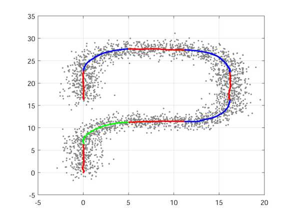
Fig. 1. Adaptive estimation of a moving object trajectory

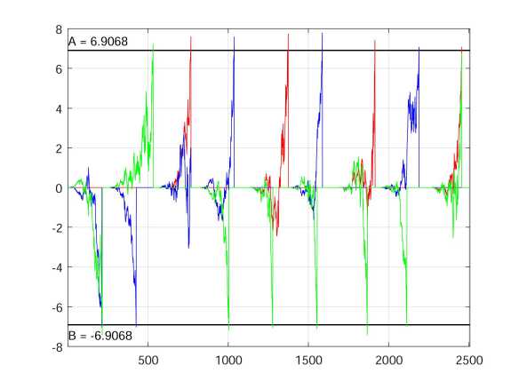
Fig. 2. Mode detection process

Level             RMSE x i x 1        x 2        x 3        x 4	nRMSE
1)  0,2273  0,0404  0,2038  0,0377 2)  0,2926  0,0449  0,2399  0,0408 3)  0,3791  0,0575  0,3440  0,0568	0,3103 0,3832 0,5182

are coloured according to detected motion mode: straight motion is painted in red, left turn is painted in blue, and the right turn is painted in green.

Fig. 2 shows a mode detection process for Example 1 given the third level of uncertainty (2). The calculated values of likelihood ratios λ k,ij are coloured according to the corresponding motion mode: straight motion mode is painted in red, left turn mode is painted in blue, and right turn mode is painted in green. We can see which motion mode has been detected on each piece of the trajectory.

Having analyzed the obtained numerical results presented in Table and illustrated in Figure, we make a few conclusions. First, for each component of the state vector x the quality of calculated estimates is good (RMSE x _i , i = 1, . . . , 4 is small enough). Second, the motion modes were detected correctly in all three considered cases, even when the level of the measurements noise is high enough.

Thus, the proposed Algorithm (ATE) of adaptive estimating moving object trajectory allows to detect correctly the motion mode and simultaneously calculate optimal linear estimates of the state vector x. Therefore, it can be recommended for solving practical tracking problems in real-life applications.

Conclusions

In the present paper, a new algorithm ATE for adaptive estimation of a moving object trajectory is proposed. The novelty of this algorithm is that it combines the hybrid linear stochastic model of an object moving along a complex trajectory with Kalman filtering and a sequential hypothesis testing. It is supposed that at known moments of time an object may change its motion to one of three possible modes. Such an approach may be used, for example for ground and marine objects tracking. The proposed algorithm was implemented in MATLAB and its efficiency was confirmed by multiple numerical experiments. Further, it will be extended to the general case when moments of changes in the motion mode are unknown.

Acknowledgements. This work was supported by the Russian Foundation for Basic Research (grants 16-41-730784, 18-37-00220).