Adaptive model for dynamic and temporal topic modeling from big data using deep learning architecture

Author: Ajeet Ram Pathak, Manjusha Pandey, Siddharth Rautaray
Journal: International Journal of Intelligent Systems and Applications @ijisa
Article in issue: 6 vol.11, 2019.
Free access
Due to freedom to express views, opinions, news, etc and easier method to disseminate the information to large population worldwide, social media platforms are inundated with big streaming data characterized by both short text and long normal text. Getting the glimpse of ongoing events happening over social media is quintessential from the viewpoint of understanding the trends, and for this, topic modeling is the most important step. With reference to increase in proliferation of big data streaming from social media platforms, it is crucial to perform large scale topic modeling to extract the topics dynamically in an online manner. This paper proposes an adaptive framework for dynamic topic modeling from big data using deep learning approach. Approach based on approximation of online latent semantic indexing constrained by regularization has been put forth. The model is designed using deep network of feed forward layers. The framework works in an adaptive manner in the sense that model is extracts incrementally according to streaming data and retrieves dynamic topics. In order to get the trends and evolution of topics, the framework supports temporal topic modeling, and enables to detect implicit and explicit aspects from sentences also.
Aspect detection, big data, deep learning, latent semantic indexing, online learning, regularization, topic modeling
Short address: https://sciup.org/15016598
IDR: 15016598 | DOI: 10.5815/ijisa.2019.06.02
Text of the scientific article Adaptive model for dynamic and temporal topic modeling from big data using deep learning architecture
Published Online June 2019 in MECS
The emergence of social media platforms lead to increase in posting of text in the form of reviews, opinions on the web, and heavily contribute for unprecedented growth of big data [1]. Many natural language processing applications such as summarization, user profiling, product recommendation, event tracking, text classification, collaborative filtering, similarity finding, sentiment analysis, etc. need to discover latent semantic topics from large text corpora. In such applications, topic modeling is the foremost step. Extracting the latent topics at large scale is challenging due to sparseness of text, spelling and grammatical errors, slangs, or jargons, unstructured data, and interrelated data discussed under different domains, etc.
Microblogging sites such as Twitter, Tumblr, Pinterest, Reddit, Yammer, etc stream large amount of short and long normal texts with substantial growth in due course of time. Streaming data are characterized by temporal order. Temporal information is necessary to get the notion of evolution and spread of domain-specific latent topics. Moreover, instead of processing large collection of time-stamped datasets with using off-line fashion in batch mode; it is more crucial for many natural language applications to analyze, summarize and extract valuable insights on the go in an online manner. Batch algorithms are not suitable for extracting topics from large scale and streaming data. Also such algorithms need to repeatedly scan the data for topic learning and need to keep the model up-to-date when new data arrives. Therefore, online algorithms are preferred for topic learning.
Online algorithms are able to handle large scale data efficiently since they only store small chunks of data for updating the model when new data arrives. This makes them more efficient than batch counterparts. For example, due to some worldwide event, many social media platforms gets flooded with comments of people, news feeds, etc and this requires automated systems to extract and track current topics of specific interest and identify emerging trends discussed on social media platforms. If extracted topics correspond to suspicious activities or alarming scenarios, then quick actions can be taken by authorized personnel for proactive measures. Hence, use of temporal topic model which works in online mode to infer dynamically generated topics from streaming data is the need of the hour.
Considering all the aforementioned motivation, this paper proposes an adaptive Framework for deep learning based dynamic and temporal topic modeling from big data. The proposed approach works in online manner for topic modeling and therefore, it is intrinsically scalable to large datasets. The work is contributed as follows.
-
• We have proposed a deep learning model for detection of dynamically generated topics from streaming data by online version of Latent Semantic Indexing (LSI) constrained by
regularization.
-
• The approach is scalable to large collection of datasets. It is flexible to support both long normal text and short text for modeling the topics.
-
• The model is adaptive and it is updated incrementally and performs temporal topic modeling to get notion of evolution and trends of topics over time.
-
• It supports extraction of implicit and explicit topics from sentences also.
The rest of the paper is portrayed as follows. Section II deals with discussion of conventional topic models, topics models based on deep learning paradigm and relation of the existing work with the proposed approach. Section III focuses on statistical environment, proposed architecture and algorithms for dynamic and temporal topic modeling and user query evaluation. The experimentation details encompassing exploratory data analysis and correspondence analysis and results are discussed in section IV. Section V gives conclusion and future directions of the research.
-
II. Related Work
Topic modeling is a statistical technique and provides automated approach for extracting latent semantic topics from documents. In classical settings, document is considered as a mixture of latent topics i.e. multinomial distribution over topics and topic is viewed as probability distribution over words.
Topic Modeling algorithms have been extensively developed for text analysis since the past decade [2]. Manually identifying the topics is not efficient and scalable due to huge size of data, wide variation, and dynamically changing nature of topics. Therefore, topic models such as Latent Dirichlet Allocation (LDA) [3], probabilistic Latent Semantic Analysis (PLSA) [4], and Latent Semantic Indexing (LSI) [5] have been put forth for automatically extracting the topics at large scale. Various topic modeling algorithms have been used for inferring the hidden topics from short texts [6-8] and normal long texts [9-10].
LDA model put forth by Blei et al. [3] is the most popular probabilistic generative model for topic modeling. Approximate technique namely convexity-based variational method is used for inference since exact inference is intractable. For estimating Bayes parameters, expectation maximization algorithm is used in LDA model. Due to probabilistic and modular nature, LDA models can be easily fit into complex architectures. This property is not supported by LSI [5] model.
LSI model [5] uses Singular Value Decomposition (SVD) to capture variance in the document collection. This approach captures implicit semantic structure among the terms in documents for identifying relevant documents based on terms present in queries. It maps high dimensional count vectors to lower dimensional latent semantic space.
The improved version of standard latent semantic analysis model has been put forth in [4]. Probabilistic latent semantic analysis model - PLSA (aspect model) follows statistical latent class model, and it is an unsupervised learning method. A method for generalization of maximum likelihood estimation, namely, tempered expectation maximization has also been proposed in [4].
Many topic modeling approaches have been put forth by modifying basic topic models like LDA, PLSA, and LSI. Hoffman et al. [11] extended LDA by proposing online variational Bayes (VB) algorithm for topic modeling over streaming data.
Scaling to large dataset of document collection is one of the most challenging tasks in topic modeling. Topic modeling approaches based on LDA and LSI pose challenges related to scalability when such methods are employed to solve real-world tasks. For an instance, it is very difficult to update term-topic matrix simultaneously for satisfying the criterion of probability distribution when the dataset is large. In case of LSI, due to orthogonality assumption, problem needs to be solved using SVD, and it is difficult to parallelize the procedure for SVD. Also topic models like LDA and PLSA assumes document as a mixture of topics and models documentlevel word co-occurrences. Wang et al. [12] came up with novel model based on regularized latent semantic indexing (RLSI) for scalable topic modeling. RLSI is different from LSI method. It uses regularization to constrain the solutions instead of using orthogonality as adopted by LSI techniques.
The online version of LDA has been put forth in [13]. This approach works on non-Markovian Gibbs sampling. The weight-matrix history is maintained in the generative process of the method according to homogeneity of domain. It does not handle inter-topic differences and drifts within same topics. Topic model for temporally sequenced data has been proposed in [14]. This model dynamically predicts future trends for data and is scalable in nature.
Some topic modeling approaches assume that words have equal weights. This results into selection of topics having highest frequency of terms in documents. But, this may cause selection of meaningless words like domainspecific stop words which are not useful for further processing. Li et al. addressed this issue by proposing conditional entropy based term weighing scheme in which entropy is measured by word co-occurrences [15]. To infer more effective topics during topic inference phase, meaningless words are assigned lower weights and informative words are assigned higher weights. This scheme is applied with Dirichlet Multinomial Mixture (DMM) model [8] and LDA model [3] to infer topics from shorts texts and normal long texts respectively.
Kuhn put forth structural topic modeling approach and captured correlation among topics pertaining to single domain [16]. Brody and Elhadad [17] employed unsupervised approach for aspect detection. They used local version of LDA working at sentence level and assumed each sentence as a document.
With success of deep learning approaches in computer vision tasks [18-20], deep learning models have also been devised for natural language processing tasks. Language model based on recurrent neural network (TopicRNN) [21] follows semi-supervised approach to capture syntactic dependency and semantic dependency of document using RNN and latent topic model respectively. This model can be considered as alternative to LDA for topic modeling. Li et al. [22] used an attention mechanism of neural networks for modeling contents and topics to recommend the hashtags.
Generative topic models usually do not consider the contextual information while performing the task of topic extraction. A Document Informed Neural Autoregressive Distribution Estimator (iDocNADE) [23] takes into account the contextual information using language models having backward and forward references. LDA-based generative topic model proposed in [24] performs incremental updating of parameters over consecutive windows, and enables faster processing by adaptive window length.
Word embeddings have found to be useful for distributed representation of words and capturing semantic and syntactic information in many natural language processing tasks such as parts-of-speech tagging, parsing, named entity recognition, etc. Enlightened by same, word embedding models have also been used for topic modeling. Zhang et al. [25] used word2vec embedding model for feature extraction from large range of bibliometric data and coupled it with k-means algorithm for improving the performance of topic extraction. Topic modeling approaches working on short texts from social media platforms suffer from data sparsity, noisy words and word sense disambiguation problems. Gao et al. [26] addressed the issue of word sense disambiguation by utilizing local and global semantic correlation provided by word embedding model. Conditional random field is used in inference phase for short text modeling. Approach in [27] introduced common semantic topic model designed using mixture of unigram models for capturing the semantic and noisy words from short texts. Weibull distribution based hybrid autoencoding inference process for deep LDA has been put forth in [28] to get hierarchical latent representation of big data for scalable topic modeling.
Considering the relation of proposed work with the existing literature, this paper proposes scalable topic modelling approach based on deep learning. The proposed model has capability to infer the dynamic topics from streaming data and provides notion of evolution and trends of topic over time.
-
III. Methodology
This section describes statistical environment and proposed architecture for topic modeling.
-
A. Statistical environment
Following matrices are used in the proposed approach.
-
• Terms Г, Г £ ^ м
г= [г,г2,..гм]
where M denotes number of terms.
-
• Sentences $ /
Sentences can be represented as set of terms
$/ = [Г1,Г2,..Г7]
where i = 1,2,.., Р and P is number of sentences. The number of terms J in a sentence are less than total number of terms i.e. J < M.
-
• Topics Ui , Ui £ ^x 1
Ui = {UVU2, ^,UK3
where i = {1,2,.., K} and K denotes number of topics.
-
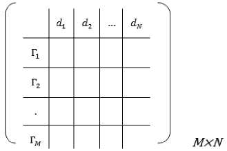
• Term-document Matrix D , D £ ^ MxW
0 = [d i, ^2, ■", ^jv]
where M denotes number of terms, and N denotes number of documents. The values in term-document matrix are calculated using TF-IDF score.
-
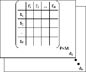
• Sentence-term matrix W, W £ ^ PxMxV
W = [w1,w2,..wN]
where P denotes number of sentences, M denotes number of terms and N denotes number of documents. For documents d 1 , d 2 ,^,d v , sentence-term matrix W is shown as three dimensional matrix. The values in sentence-term matrix ‘W’ are calculated using 2 ways.
-
- Presence or absence of terms in each sentence can be represented by 1 or 0 respectively in sentenceterm matrix
-
- Term frequency–inverse document frequency (TF-IDF) score can be used for calculating the values in a sentence-term matrix
where K denotes number of topics, N denotes number of documents, vk „denotes weight of kh topic in document dN . As shown in term-document matrix, each column v1,v2, ^vn gives the representation of document d 1 , d 2 , ... Vv in the topic space.
^ N
u 1
v 12
v1n
U 2
-
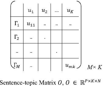
• Term-topic matrix U , UE ^^
where M is number of terms, K is number of topic. Entries in the term-topic matrix correspond to the weight of m th term in topic ‘ k’ which is denoted by um. . At sentence level, term Г gives name of the aspect if term belongs to the topic i.e. corresponding weight of the term umк is higher for the given topic ut . Term-topic matrix shows strength of belongingness of each term to topic.
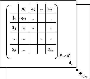
0 = [o1,o2,^,oN]
where P denotes number of sentences, K denotes number of topics and N denotes number of documents. For documents d 1 ,d 2 ,...,dN , three dimensional sentencetopic matrix is shown where qp k denotes weight of each kth topic in a sentence.
-
• Topic-document Matrix V, V E K ^xv
V = [v^v,...,^]
u К vk1 vk2 • vkn )
v 1 v 2 .. v n
t t t A
Each column v 1 , v 2 ,..,v n gives representation of document d 1 , d 2 ,..,d N respectively in topic space
-
B. Proposed architecture
Fig. 1 shows the proposed methodology of topic modeling. The architecture is divided into 4 main modules. The model works on steaming data. For building the prototyped model, we collected the dataset. Initially, data cleaning and tokenization has been performed using R, Python and SpaCy packages. After data preprocessing, exploratory data analysis (EDA) and correspondence analysis (CA) has been performed. EDA is used to infer useful information from data, understand the behaviour of data and check usefulness of data for further phase of topic modelling.
We have done correspondence analysis as a generalization of principal component analysis (PCA), and SVD. We analysed the data using heat map, scree plots, factor score and most contributing variable. We designed the topic model for temporal analysis by online latent semantic indexing constrained by regularization using deep learning approach. We designed the model using dense network of feed forward network layers.
Use of sentence level topic modeling yields to detect both implicit and explicit topics mentioned in sentences. We applied algorithm 1 for training the model incrementally.
Due to online learning, only one document remains in memory at a time. Therefore space complexity is given by DocLength + К where DocLength stands for document length and K is number of topics. For initial construction of ‘U’ and ‘V’ matrices, space complexity is D o cL egg th x N + NN. For processing document at time t , the time for updating ‘U’ and ‘V’ matrices as shown in equation (3) is significant, therefore, time complexity is given by C x M x К 2 where C denotes number of times the algorithm iterated, M is number of terms and K is number of topics.
When user sends a query for inferring the topics, algorithm 2 is followed. The topics associated with terms mentioned in query and other implied latent topics are returned by model as output of the query evaluation.
-
■ Data cleaning
-
■ Data tokenization
Documents 1,2,..,N

Streaming data
Preprocessing
Preprocessing using R, Python and SpaCy packages for enhancing the effectiveness of data
Exploratory Data Analysis
-
■ Correspondence Analysis as a generalization of PCA
-
■ Singular Value Decomposition
-
■ Analysis using heat map, scree plots, factor score
EDA to infer useful information from data, understanding the behavior of data, checking usefulness of data for further phase of topic modeling and improving the analysis
Input user query
Topic Modeling by Online version of Latent Semantic Indexing

■ ■ ■
■
■ ■
■
■
constrained by regularization
Find the distribution of documents
Calculate TF-IDF score for terms in document collection
Draw Term-document matrix ‘D’ and sentence-term matrix ‘W’ for each document.
Approximate the Term-document matrix ‘D’ as a product of Termtopic Matrix ‘U’ and Topic-document matrix ‘V’
Based on ‘U’ and ‘V’, matrices draw sentence-topic matrix ‘O’ Minimize the difference between actual document and approximated representation of document by regularization For each document collected at time t, update the matrices ‘U’ and ‘V’
Retrieve the term topic matrix ‘U’
■ ■
■
■
■
Input Query Processing
Analyze the query
Retrieve terms explicitly mentioned in the query
Perform explicit topic detection with the help of term topic matrix ‘U’
If term is not explicitly mentioned in the input query, then consult sentence-term matrix ‘W’ and sentence-topic matrix ‘O’ for implicit detection of topics.
Choose top topics having highest scores/weights
Evaluation of user queries on streaming data to infer dynamic topics
Dynamic topic modeling (Topics are updated using online learning)
d N
d 1
Topic 1
Topic 2
Topic K
Dynamically generated topics
Fig.1. Proposed architecture for topic modeling
Algorithm 1: Temporal Topic Modeling by Online Latent Semantic Indexing constrained by regularization
Model Training
Input: Streaming Data
Output: Trained model obtained using online learning
-
• Find the distribution of documents dY, d2, ..., dN.
-
• Calculate TF-IDF score for terms in document collection using equation (1).
TF1DF = ^) x log -—(1)
|d| |{deDTed}| where, с (Г, d) is a count that term Г occurs in document d, |d| is Length of document d, |D| is Total count of documents in document collection, and |{d ЕД:Г £ d}| is total count of documents in which term Г occurs
-
• Draw term-document matrix ‘D’ and sentenceterm matrix ‘W’ for each document.
-
• Approximate term-document matrix ‘D’ as a product of term-topic Matrix ‘U’ and topicdocument matrix ‘V’ .
dn ~ Uvn (2)
where du is document, 'U' is term-topic matrix, vn is Representation of document du in the topic space.
-
• Based on ‘U’ and ‘V’ matrices, draw sentencetopic matrix ‘O’ .
-
• Minimize the difference between actual document and approximated representation of document by 12 regularization according to Eq. (3)
Мг-UvX (3)
-
• For each document collected at time t , update the matrices ‘V’ and ‘U’ by approximating latent semantic indexing model using Eq. (3).
-
• Retrieve the term topic matrix ‘U’ and topicdocument matrix ‘V’
Algorithm 2: Query Evaluation
Input: User Query
Output: Dynamically generating topics
-
• Analyze the query
-
• Retrieve terms explicitly mentioned in the query
-
• Perform explicit topic detection with the help of term topic matrix ‘U’
-
• If term is not explicitly mentioned in the input query, then consult sentence-term matrix ‘W’ and sentence-topic matrix ‘O’ for implicit detection of topics.
-
• Choose top topics having highest scores/weights
-
IV. Experimentation Details
count of words discussed under the hashtags #ethereum, #facebook and #bitcoin respectively in tweets per week.
For topic modeling, real word dataset related to 3 hashtags has been collected using Twitter APIs. Tweets associated with the hashtags #bitcoin, #ethereum, and #facebook are captured from 3-3-2018 to 3-5-2018. Tweets are analyzed weekly according to the duration of data collected. For experimentation, Python, and R programming languages have been used. We also used SpaCy for advanced natural language processing task and developed the model in the TensorFlow framework.
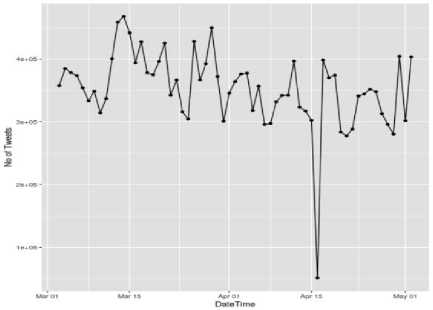
(a) #ethereum
Based on the collected dataset in .csv format having 3 major hashtags, we converted the duration into weeks i.e. from 9 to week 18 of the year. Out of 22 attributes of the dataset ( viz. 'Tweet ID, Conversation ID, Author Id , Author Name, isVerified, DateTime, Tweet Text, Replies, Retweets, Favorites, Mentions, Hashtags, Permalink, URLs, isPartOfConversation, isReply, isRetweet, Reply To User ID, Reply To User Name, Quoted Tweet ID, Quoted Tweet User Name, Quoted Tweet User ID' ), we only focused on attributes - DateTime , Tweet Text and Hashtags . The reason behind choosing these 3 attributes out of 22 attributes is that our aim is to perform temporal topic modeling from Tweet text to get the notion of evolution and trends of topics discussed under various hashtags over time. Therefore, we are considering 3 attributes ( DateTime , Tweet Text and Hashtags ) for topic modeling.
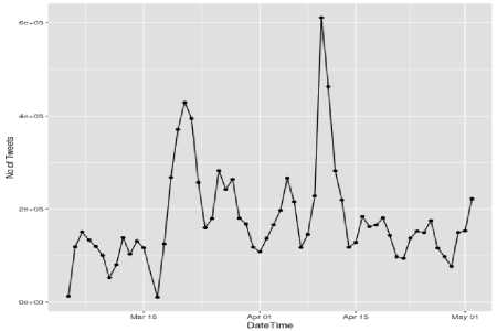
(b) #facebook
-
A. Exploratory Data Analysis
As a first step towards topic modeling, Exploratory Data Analysis has been performed. All the steps in EDA have been carried out on aforementioned dataset having 3 main hashtags. The main objective of EDA is to understand how much useful information does dataset hold. Therefore, we first calculated the five-number summary statistics for the ‘ DateTime’ attribute to
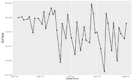
(c) #bitcoin
Fig.2. Frequency of words against each month for (a) #ethereum, (b) #facebook, and (c) #bitcoin (X-axis represents time in terms of date and Y-axis represents count of tweets)
understand the distribution of words over weeks. After that we calculated frequency of words against each month. Fig. 2 - (a), (b) and (c) shows the frequency of words against each month from March, to May for hashtags #ethereum, #facebook and #bitcoin respectively. Frequency of occurrence of words is calculated using Eq. (4). Table 1 shows the frequency of words based on weeks.
Frequency = ------- (4)
Table 1. Weekly Frequency of Words for #Ethereum
|
week |
word |
free; |
n |
total |
|
9 |
#ethereum |
0.039225512 |
29118 |
742323 |
|
9 |
#eth |
0.033369571 |
24771 |
742323 |
|
9 |
#btc |
0.028740858 |
21335 |
742323 |
|
9 |
#bitcoin |
0.028646560 |
21265 |
742323 |
|
9 |
#ico |
0.023175895 |
17204 |
742323 |
|
9 |
#blockchain |
C02273134c |
16874 |
742323 |
|
9 |
#cryptocurr |
0.022020064 |
16346 |
742323 |
tоtaI wоrds where n denotes number of times specific word occurs in a week, total_words denote total number of words appeared in a week.
To get clear notion of appearance of words in corresponding weeks, tables 1, 2 and 3 show the count and frequency of words weekly for the hashtags #bitcoin, #ethereum, and #facebook respectively. From tables 1, 2 and 3, it can be observed that value of frequency is very low. This is the major issue related to big data. To overcome this issue, correspondence analysis has been done considering the count of terms occurred in a week instead of frequency of terms. Tables 4, 5 and 6 show the
Table 2. Weekly Frequency of Words for #Facebook
|
week |
word |
freq |
n |
total |
|
9 |
|
0.073163210 |
949 |
12971 |
|
9 |
|
0.012335209 |
160 |
12971 |
|
9 |
|
0.011795544 |
153 |
12971 |
|
9 |
en |
0.009251407 |
120 |
12971 |
|
9 |
de |
0.008711742 |
113 |
12971 |
|
9 |
|
0.007246935 |
94 |
12971 |
|
9 |
#socialmedia |
0.006475985 |
84 |
12971 |
Table 3. Weekly Frequency of Words for #Bitcoin
|
week |
word |
freq |
n |
total |
|
9 |
#bitcoin |
0.067669116 |
26952 |
398291 |
|
9 |
#cryptocurr |
0.023540577 |
9376 |
398291 |
|
9 |
#blockchain |
0.021306030 |
8486 |
398291 |
|
9 |
ffethereum |
0.020575408 |
8195 |
398291 |
|
9 |
#crypto |
0.019721761 |
7855 |
398291 |
|
9 |
#btc |
0.018283115 |
7282 |
398291 |
-
B. Correspondence Analysis
For extracting useful information from dataset which is represented using contingency table, reducing the data by focusing on important information and analyzing the patterns in data, we have performed singular value decomposition and decomposition of positive semidefinite matrices. For handling the qualitative variables, Principal Component Analysis has been generalized as Correspondence Analysis [29].
This would mean that something important happened during that week that brought different words closer to each other, and therefore, we are just using highest frequency word as topic.
For CA, the whole dataset with 3 hashtags, namely, #ethereum, #facebook and #bitcoin and associated terms have been displayed in row-column manner in which rows represent terms associated with hashtags and columns represent weeks. Entries in contingency table represent how many times the given terms have been discussed on Twitter in a given week. Table 7 shows contingency table of terms associated with 3 hashtags along with their occurrence in weeks from 9 to 18.
-
1) Singular Value Decomposition
For reducing data size, SVD finds new components which are derived from original variables using linear combinations. The first component exhibits as much as large variance as possible. This component explains the largest part of inertia of table. Subsequent principal component is obtained having large variance with a constraint that it is orthogonal to the preceding component. These new variables used for deriving the components are called as factor scores. Factor scores can be assumed as projections of observed data onto the principal components. We have used Correspondence Analysis via ExPosition. To reduce dimensions, we used SVD, and got new axis for all weeks as shown in the table 8.
-
2) Heat Map Analysis
It can be noted from histogram that count of terms #bitcoin1, #ethereum, and #facebook is very high (shown in red color) compared to other terms.
-
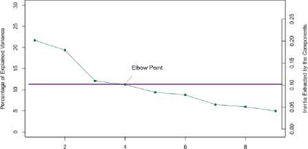
3) Scree Plots
As we only need to infer the useful information, the problem is how many components need to be considered for correspondence analysis. Scree plots give an intuition which components represent data in best possible way. Scree plots may or may not give best components since this procedure is somewhat subjective.
For scree plot analysis, Eigen values are plotted according to their size. Then an elbow point is decided such that slope of graph becomes flat from steep one. The points before this elbow point are kept for further analysis. These points represent the data in best possible manner. Three points above elbow point best represent the data as shown in figure 4. Based on scree plot, only two dimensions possessing large amount of data variability are selected for further analysis.
-
4) Factor Scores
Factor scores represent the proportion of the total inertia ‘‘explained’’ by the dimension. Factor score obtained from scree plot asymmetrically and symmetrically for both dimensions are plotted in figures 5 and 6 respectively where л represents Eigen values and т represents percentage of data explained by the dimension.
Table 4. Weekly Frequency of Words for #Ethereum
|
Word |
9 |
10 |
11 |
12 |
13 |
14 |
15 |
16 |
17 |
18 |
|
#ada |
4909 |
8017 |
22093 |
8335 |
7913 |
4790 |
4459 |
5966 |
5662 |
3024 |
|
#airdrop |
8803 |
26098 |
52520 |
35142 |
36588 |
23695 |
23437 |
17425 |
22093 |
10432 |
|
#altcoin |
5252 |
15007 |
20565 |
19074 |
24754 |
15769 |
16140 |
15630 |
14965 |
7212 |
|
#bch |
1676 |
5532 |
0 |
0 |
5837 |
4847 |
0 |
4335 |
6812 |
3517 |
|
#binanc |
2100 |
6885 |
5777 |
6301 |
5311 |
5388 |
6872 |
4604 |
8544 |
3573 |
|
#bitcoin |
21265 |
74625 |
86687 |
80112 |
88349 |
80468 |
78405 |
75880 |
74117 |
35899 |
|
#bitcoincash |
0 |
0 |
0 |
0 |
0 |
0 |
0 |
5292 |
7042 |
4591 |
|
#blockchain |
16874 |
63634 |
77100 |
76298 |
86977 |
73230 |
74537 |
62033 |
70407 |
33964 |
|
#bounti |
4349 |
13399 |
23040 |
18379 |
23916 |
12641 |
15873 |
12443 |
12209 |
4913 |
|
#btc |
21335 |
63269 |
85576 |
62158 |
66565 |
55042 |
56945 |
48847 |
55188 |
25308 |
|
#bts |
0 |
0 |
0 |
5602 |
0 |
0 |
0 |
4577 |
0 |
0 |
|
#coin |
0 |
0 |
0 |
0 |
8583 |
4176 |
0 |
0 |
0 |
0 |
|
#crowdfund |
1649 |
0 |
0 |
0 |
0 |
0 |
6617 |
4170 |
4572 |
0 |
|
#crowdsal |
0 |
4511 |
0 |
5034 |
4876 |
5252 |
6068 |
4020 |
4487 |
0 |
|
#crypto |
16057 |
49975 |
64539 |
57773 |
64473 |
57169 |
63050 |
54821 |
60671 |
28176 |
|
#cryptocurr |
16346 |
55146 |
67646 |
65178 |
72530 |
64913 |
65206 |
60007 |
58497 |
27540 |
|
#cryptonew |
0 |
0 |
0 |
4878 |
0 |
4196 |
4725 |
0 |
0 |
0 |
|
#dash |
2216 |
6034 |
6165 |
6053 |
6340 |
6508 |
4518 |
4540 |
5847 |
2968 |
|
#digitizecoin |
0 |
0 |
0 |
0 |
0 |
0 |
4733 |
0 |
0 |
0 |
|
#earn |
0 |
0 |
0 |
0 |
5741 |
0 |
0 |
0 |
0 |
0 |
|
#elsalvador |
0 |
0 |
0 |
0 |
0 |
0 |
0 |
0 |
0 |
3205 |
|
#energytoken |
5921 |
8852 |
0 |
0 |
0 |
0 |
0 |
0 |
0 |
0 |
|
#eo |
4481 |
9439 |
0 |
4646 |
6158 |
4802 |
0 |
4102 |
8049 |
4669 |
|
#erc20 |
1385 |
0 |
5729 |
6245 |
7331 |
4942 |
4706 |
4441 |
5897 |
3412 |
|
#escort |
0 |
0 |
0 |
0 |
0 |
0 |
0 |
3786 |
0 |
3628 |
|
#etc |
1643 |
6167 |
0 |
0 |
0 |
0 |
0 |
0 |
0 |
0 |
|
#eth |
24771 |
74637 |
99115 |
77422 |
87220 |
71144 |
73107 |
58282 |
67597 |
32730 |
|
#ether |
3120 |
11848 |
13683 |
14143 |
18291 |
19046 |
16220 |
11351 |
11154 |
5596 |
|
#ethereum |
29118 |
108179 |
123037 |
114655 |
121189 |
113522 |
110730 |
99528 |
100171 |
48708 |
|
#fintech |
0 |
0 |
0 |
0 |
0 |
0 |
0 |
0 |
3928 |
0 |
|
#xrp |
9686 |
26943 |
24497 |
20066 |
19455 |
17269 |
16319 |
14031 |
22588 |
10513 |
|
#xvg |
5386 |
10978 |
30172 |
11820 |
9724 |
6645 |
5888 |
8167 |
5656 |
3131 |
|
airdrop |
3652 |
8952 |
17883 |
10533 |
7212 |
6779 |
7201 |
4515 |
6496 |
2585 |
|
blockchain |
0 |
0 |
0 |
4972 |
4746 |
4063 |
4967 |
4187 |
4662 |
0 |
|
btc |
4896 |
16187 |
15886 |
18275 |
16913 |
14503 |
16235 |
14673 |
18964 |
9716 |
|
chanc |
0 |
0 |
10243 |
0 |
0 |
0 |
0 |
0 |
0 |
0 |
|
crypto |
0 |
5167 |
0 |
4677 |
4995 |
4536 |
4821 |
4134 |
4342 |
0 |
|
cryptocurr |
0 |
0 |
0 |
0 |
0 |
0 |
4375 |
0 |
0 |
0 |
|
de |
0 |
0 |
0 |
0 |
0 |
0 |
0 |
0 |
0 |
3674 |
|
earn |
2223 |
5665 |
0 |
0 |
0 |
0 |
0 |
0 |
0 |
0 |
|
eth |
2629 |
8605 |
8347 |
9307 |
8228 |
6775 |
6539 |
5530 |
6726 |
3568 |
|
free |
4869 |
12371 |
22354 |
9599 |
5688 |
4401 |
4254 |
0 |
0 |
0 |
|
friend |
1510 |
0 |
11701 |
0 |
0 |
0 |
0 |
0 |
0 |
0 |
|
goal |
0 |
0 |
9690 |
0 |
0 |
0 |
0 |
0 |
0 |
0 |
|
ico |
0 |
4522 |
0 |
5096 |
0 |
4069 |
5552 |
3911 |
0 |
0 |
|
join |
5105 |
15739 |
15012 |
11259 |
10457 |
8495 |
8946 |
7508 |
6947 |
2836 |
|
link |
0 |
0 |
8352 |
5435 |
0 |
0 |
0 |
0 |
0 |
0 |
|
mani |
0 |
0 |
10111 |
0 |
0 |
0 |
0 |
0 |
0 |
0 |
|
offer |
0 |
0 |
5691 |
0 |
0 |
0 |
0 |
0 |
0 |
0 |
|
peopl |
0 |
0 |
10731 |
0 |
0 |
0 |
0 |
0 |
0 |
0 |
|
platform |
0 |
4424 |
0 |
4653 |
4636 |
4337 |
4483 |
3521 |
0 |
0 |
|
price |
0 |
4429 |
0 |
0 |
4457 |
0 |
0 |
0 |
0 |
0 |
|
project |
2154 |
8793 |
19084 |
11368 |
10908 |
10298 |
10595 |
8079 |
8053 |
3245 |
|
reach |
0 |
0 |
9778 |
0 |
0 |
0 |
0 |
0 |
0 |
0 |
|
refer |
0 |
0 |
5695 |
0 |
0 |
0 |
0 |
0 |
0 |
0 |
|
regist |
0 |
0 |
13344 |
4883 |
0 |
0 |
0 |
0 |
0 |
0 |
|
share |
0 |
0 |
14946 |
4499 |
0 |
0 |
0 |
0 |
0 |
0 |
|
start |
0 |
0 |
7559 |
0 |
0 |
0 |
0 |
0 |
0 |
0 |
|
time |
0 |
0 |
7462 |
4589 |
0 |
0 |
0 |
0 |
0 |
0 |
|
token |
4541 |
13866 |
41710 |
19947 |
13665 |
11690 |
13544 |
7998 |
11945 |
4653 |
Table 5. Weekly Frequency of Words for #Facebook
|
Word |
9 |
10 |
11 |
12 |
13 |
14 |
15 |
16 |
17 |
18 |
|
#actu |
33 |
1887 |
1719 |
0 |
2248 |
2178 |
0 |
2046 |
2078 |
1070 |
|
#amazon |
0 |
985 |
706 |
0 |
0 |
0 |
0 |
0 |
1223 |
0 |
|
#busi |
29 |
1283 |
1041 |
0 |
0 |
0 |
0 |
1566 |
1457 |
712 |
|
#cambridgeanalyt |
0 |
0 |
0 |
5004 |
1658 |
0 |
0 |
0 |
0 |
0 |
|
#cambridgeanalytica |
0 |
0 |
780 |
13947 |
4700 |
4102 |
6515 |
1851 |
1307 |
826 |
|
#congress |
0 |
0 |
0 |
0 |
0 |
0 |
2309 |
0 |
0 |
0 |
|
#data |
0 |
0 |
0 |
3958 |
2986 |
2558 |
3721 |
1867 |
1233 |
0 |
|
#date |
0 |
0 |
0 |
0 |
0 |
0 |
0 |
0 |
0 |
832 |
|
#deletefacebook |
0 |
0 |
0 |
5732 |
3050 |
1797 |
2762 |
0 |
0 |
0 |
|
#digitalmarket |
0 |
895 |
710 |
0 |
0 |
0 |
0 |
1356 |
1218 |
0 |
|
#f8 |
0 |
0 |
0 |
0 |
0 |
0 |
0 |
0 |
0 |
1318 |
|
|
949 |
50748 |
41961 |
130670 |
86932 |
76678 |
128772 |
63718 |
57189 |
32773 |
|
#facebookdatabreach |
0 |
0 |
0 |
0 |
1635 |
0 |
2683 |
0 |
0 |
0 |
|
#facebookdataleak |
0 |
0 |
0 |
0 |
0 |
0 |
2801 |
0 |
0 |
0 |
|
#facebookg |
0 |
0 |
0 |
3196 |
0 |
0 |
0 |
0 |
0 |
0 |
|
#faitsdiv |
33 |
1882 |
1717 |
0 |
2241 |
2173 |
0 |
2037 |
2069 |
1067 |
|
#follow |
18 |
0 |
0 |
0 |
0 |
0 |
0 |
0 |
0 |
0 |
|
#gdpr |
0 |
0 |
0 |
0 |
0 |
0 |
0 |
1499 |
0 |
0 |
|
#googl |
42 |
2779 |
2532 |
4691 |
5555 |
3372 |
4228 |
3154 |
3154 |
1144 |
|
#hiphop |
21 |
1249 |
950 |
0 |
0 |
0 |
0 |
0 |
1102 |
0 |
|
#info |
35 |
1918 |
1747 |
2435 |
2295 |
2217 |
0 |
2101 |
2118 |
1077 |
|
|
153 |
7778 |
5601 |
8764 |
7736 |
7760 |
8403 |
7887 |
7987 |
3791 |
|
#justic |
35 |
1962 |
1773 |
2452 |
2316 |
2263 |
2288 |
2205 |
2266 |
1125 |
|
|
23 |
1091 |
948 |
0 |
0 |
0 |
0 |
1384 |
1390 |
0 |
|
#maga |
0 |
0 |
0 |
0 |
0 |
0 |
2999 |
0 |
0 |
0 |
|
#market |
36 |
2763 |
1954 |
3032 |
2726 |
2457 |
2865 |
2591 |
2902 |
1449 |
|
#markzuckerberg |
0 |
0 |
0 |
3952 |
0 |
1805 |
7903 |
0 |
0 |
0 |
|
#music |
46 |
2458 |
2201 |
3045 |
2798 |
2846 |
3027 |
2820 |
2985 |
1497 |
|
#new |
0 |
974 |
803 |
0 |
1616 |
1734 |
0 |
1525 |
1459 |
763 |
|
le |
0 |
0 |
0 |
2617 |
1695 |
0 |
2817 |
1396 |
1059 |
834 |
|
les |
19 |
0 |
0 |
0 |
0 |
0 |
0 |
0 |
0 |
725 |
|
live |
18 |
917 |
808 |
0 |
0 |
0 |
0 |
0 |
0 |
0 |
|
los |
0 |
0 |
0 |
0 |
0 |
1652 |
0 |
0 |
0 |
0 |
|
mark |
0 |
0 |
0 |
2944 |
0 |
0 |
6420 |
0 |
0 |
0 |
|
market |
30 |
990 |
0 |
0 |
0 |
0 |
0 |
0 |
1092 |
0 |
|
media |
33 |
1383 |
1208 |
3226 |
2058 |
1885 |
3156 |
1705 |
1494 |
672 |
|
million |
0 |
0 |
0 |
0 |
0 |
1853 |
0 |
0 |
0 |
0 |
|
moment |
26 |
1072 |
964 |
0 |
0 |
0 |
0 |
1193 |
1192 |
0 |
|
news |
0 |
1296 |
827 |
0 |
1615 |
1580 |
0 |
0 |
0 |
703 |
|
page |
66 |
2644 |
2094 |
3646 |
2885 |
2674 |
3505 |
2364 |
2321 |
1154 |
|
para |
20 |
1126 |
805 |
0 |
1709 |
1636 |
0 |
1655 |
1425 |
1028 |
|
peopl |
18 |
0 |
0 |
3429 |
1921 |
2004 |
3763 |
0 |
0 |
0 |
|
person |
0 |
0 |
0 |
2847 |
0 |
0 |
0 |
0 |
0 |
0 |
|
post |
32 |
1751 |
1211 |
2450 |
2007 |
1685 |
2311 |
1629 |
1722 |
898 |
|
privaci |
0 |
0 |
0 |
2567 |
2799 |
2136 |
4267 |
1673 |
0 |
780 |
|
question |
0 |
0 |
0 |
0 |
0 |
0 |
3826 |
0 |
0 |
0 |
|
radiocapitol |
25 |
997 |
922 |
0 |
0 |
0 |
0 |
0 |
1091 |
0 |
|
scandal |
0 |
0 |
0 |
3077 |
1805 |
1632 |
0 |
0 |
0 |
0 |
|
senat |
0 |
0 |
0 |
0 |
0 |
0 |
3569 |
0 |
0 |
0 |
|
share |
0 |
0 |
0 |
2457 |
0 |
1833 |
2849 |
0 |
0 |
0 |
|
social |
60 |
2131 |
1766 |
5031 |
3234 |
2631 |
4526 |
2540 |
2228 |
1072 |
|
su |
0 |
0 |
0 |
0 |
0 |
0 |
0 |
1254 |
0 |
0 |
|
sur |
0 |
914 |
0 |
0 |
0 |
0 |
0 |
0 |
0 |
0 |
|
time |
28 |
0 |
0 |
3166 |
1627 |
0 |
2645 |
0 |
0 |
0 |
|
tip |
19 |
0 |
0 |
0 |
0 |
0 |
0 |
0 |
0 |
0 |
|
user |
0 |
0 |
0 |
4479 |
2942 |
3965 |
5084 |
2144 |
1281 |
895 |
|
video |
18 |
1236 |
766 |
0 |
0 |
0 |
0 |
0 |
1042 |
0 |
|
zuckerberg |
0 |
0 |
0 |
4690 |
1625 |
2486 |
11162 |
1224 |
0 |
763 |
Table 6. Weekly Frequency of Words for #Bitcoin
|
Word |
9 |
10 |
11 |
12 |
13 |
14 |
15 |
16 |
17 |
18 |
|
#ada |
533 |
0 |
3477 |
0 |
0 |
0 |
0 |
0 |
0 |
0 |
|
#airdrop |
2638 |
10038 |
12507 |
11880 |
7421 |
5107 |
7985 |
3490 |
3742 |
2120 |
|
#altcoin |
3324 |
12295 |
13478 |
14894 |
10800 |
7325 |
13349 |
6072 |
7680 |
3825 |
|
#bch |
580 |
0 |
0 |
0 |
0 |
1866 |
0 |
0 |
1953 |
0 |
|
#binanc |
867 |
3603 |
3463 |
4556 |
2974 |
3130 |
4372 |
2906 |
3326 |
1713 |
|
#bitcoin |
26952 |
129250 |
130504 |
142416 |
93379 |
88906 |
139196 |
70279 |
84378 |
40098 |
|
#bitcoincash |
805 |
3329 |
3176 |
3487 |
2468 |
2912 |
3852 |
2703 |
4746 |
3084 |
|
#bittrex |
0 |
0 |
0 |
0 |
0 |
0 |
0 |
1327 |
0 |
0 |
|
#blockchain |
8486 |
41274 |
44567 |
49860 |
32235 |
28574 |
45937 |
20584 |
28864 |
15041 |
|
#bounti |
1602 |
5557 |
9347 |
9114 |
5793 |
3129 |
6389 |
2043 |
0 |
1003 |
|
#btc |
7282 |
32320 |
34138 |
33660 |
24708 |
21475 |
34979 |
15436 |
21689 |
10554 |
|
#bts |
0 |
0 |
0 |
4123 |
0 |
0 |
0 |
0 |
0 |
0 |
|
#busi |
0 |
0 |
0 |
0 |
1989 |
0 |
0 |
0 |
0 |
0 |
|
#coin |
544 |
2564 |
0 |
0 |
3963 |
0 |
0 |
0 |
0 |
0 |
|
#coinbas |
674 |
0 |
0 |
0 |
0 |
1647 |
2644 |
0 |
0 |
0 |
|
#costarica |
0 |
0 |
0 |
0 |
0 |
0 |
0 |
0 |
0 |
1258 |
|
#crowdfund |
0 |
0 |
0 |
0 |
0 |
0 |
2577 |
0 |
0 |
0 |
|
#crowdsal |
0 |
0 |
0 |
2824 |
0 |
0 |
3536 |
0 |
0 |
0 |
|
#crypto |
7855 |
34970 |
36987 |
38793 |
23964 |
23958 |
39727 |
20486 |
26705 |
14038 |
|
#cryptocurr |
9376 |
42126 |
46774 |
52489 |
35009 |
30402 |
51495 |
26833 |
33424 |
16409 |
|
#cryptonew |
0 |
2919 |
2865 |
3296 |
2009 |
1834 |
3759 |
0 |
1773 |
0 |
|
#cybersecur |
2396 |
8491 |
9800 |
12639 |
9689 |
11301 |
15782 |
8265 |
4301 |
0 |
|
#dash |
645 |
2524 |
2959 |
2779 |
0 |
1904 |
0 |
1410 |
1925 |
0 |
|
#earn |
0 |
0 |
0 |
0 |
2774 |
0 |
0 |
0 |
0 |
0 |
|
#elsalvador |
0 |
0 |
0 |
0 |
0 |
0 |
0 |
0 |
0 |
1816 |
|
#eo |
0 |
0 |
0 |
0 |
0 |
0 |
0 |
0 |
2121 |
1056 |
|
#escort |
0 |
0 |
0 |
0 |
0 |
0 |
0 |
1298 |
2142 |
2168 |
|
#eth |
4133 |
15872 |
19390 |
18999 |
14174 |
11231 |
17540 |
6999 |
9486 |
4917 |
|
#ether |
1081 |
5281 |
5903 |
6822 |
5362 |
5166 |
8506 |
2842 |
3459 |
1954 |
|
#ethereum |
8195 |
37482 |
40265 |
45831 |
32256 |
27772 |
47159 |
23838 |
28119 |
15209 |
|
#vip |
0 |
0 |
0 |
0 |
0 |
0 |
0 |
0 |
0 |
1822 |
|
#xrp |
1483 |
6590 |
4916 |
5638 |
3961 |
3662 |
5279 |
3034 |
3997 |
2064 |
|
#xvg |
651 |
0 |
3361 |
3226 |
0 |
0 |
2917 |
1353 |
0 |
0 |
|
000guarium |
0 |
0 |
0 |
0 |
0 |
0 |
0 |
1311 |
0 |
0 |
|
airdrop |
620 |
0 |
0 |
0 |
0 |
0 |
0 |
0 |
0 |
0 |
|
bitcoin |
2711 |
14780 |
14408 |
13655 |
7537 |
7178 |
11675 |
5826 |
8137 |
3793 |
|
blockchain |
679 |
3830 |
3165 |
4987 |
2127 |
1920 |
3561 |
1643 |
2414 |
1368 |
|
btc |
3013 |
12069 |
13080 |
14361 |
8529 |
7151 |
11433 |
6156 |
8969 |
4928 |
|
buy |
0 |
0 |
3049 |
3092 |
2252 |
1773 |
2703 |
2144 |
2452 |
1038 |
|
crypto |
1098 |
5655 |
5945 |
5495 |
3300 |
3129 |
4997 |
2410 |
3177 |
1661 |
|
cryptocurr |
956 |
5092 |
5437 |
5222 |
3318 |
3026 |
4341 |
2091 |
2740 |
1309 |
|
de |
0 |
0 |
2536 |
2867 |
2198 |
1581 |
2924 |
2074 |
2880 |
2359 |
|
eth |
612 |
2817 |
2844 |
3870 |
0 |
0 |
2595 |
1287 |
1797 |
1191 |
|
exchang |
0 |
3077 |
0 |
2945 |
0 |
1639 |
2622 |
0 |
0 |
0 |
|
free |
939 |
4028 |
3615 |
3340 |
0 |
1680 |
0 |
1327 |
1846 |
0 |
|
hour |
0 |
0 |
0 |
0 |
0 |
1838 |
2616 |
0 |
0 |
0 |
|
ico |
0 |
2604 |
2803 |
2955 |
0 |
0 |
2969 |
1251 |
0 |
0 |
|
invest |
0 |
2545 |
0 |
0 |
0 |
0 |
0 |
0 |
0 |
0 |
|
join |
974 |
4141 |
4132 |
3385 |
2055 |
1808 |
2598 |
1706 |
1813 |
0 |
|
market |
792 |
3984 |
4242 |
4148 |
3030 |
2923 |
3997 |
1837 |
3124 |
1311 |
|
mine |
0 |
2674 |
2724 |
0 |
0 |
0 |
0 |
0 |
0 |
0 |
|
price |
1243 |
6543 |
6949 |
7200 |
4701 |
4847 |
7262 |
3282 |
4641 |
1921 |
|
project |
0 |
2565 |
2527 |
3030 |
2006 |
1927 |
2912 |
1275 |
0 |
0 |
|
secur |
564 |
0 |
0 |
0 |
0 |
0 |
0 |
0 |
0 |
0 |
|
sell |
0 |
0 |
0 |
0 |
0 |
0 |
0 |
1423 |
0 |
0 |
|
start |
0 |
2745 |
0 |
0 |
0 |
0 |
0 |
1323 |
0 |
0 |
|
telegram |
557 |
0 |
0 |
0 |
0 |
0 |
0 |
0 |
0 |
0 |
|
token |
808 |
3766 |
3547 |
3890 |
2380 |
1864 |
2717 |
1329 |
1852 |
0 |
|
trade |
730 |
3604 |
3056 |
2933 |
0 |
1966 |
0 |
1375 |
1859 |
0 |
|
world |
0 |
0 |
0 |
3240 |
0 |
0 |
0 |
0 |
0 |
0 |
Table 7. Contingency table of hashtags along with their occurrence in weeks from 9 to 18
|
Weeks |
||||||||||
|
Words |
9 |
10 |
11 |
12 |
13 |
14 |
15 |
16 |
17 |
18 |
|
|
|
|
|
|
|
|
|
|
|
|
|
▼ |
||||||||||
|
#bitcoin |
21265 |
74625 |
86687 |
80112 |
88349 |
80468 |
78405 |
75880 |
74117 |
35899 |
|
#blockchain |
0 |
63634 |
0 |
76298 |
86977 |
73230 |
74537 |
62033 |
70407 |
33964 |
|
#btc |
21335 |
63269 |
85576 |
0 |
0 |
0 |
0 |
0 |
0 |
0 |
|
#crypto |
0 |
0 |
0 |
0 |
0 |
0 |
0 |
0 |
60671 |
28176 |
|
#cryptocurr |
0 |
0 |
0 |
0 |
0 |
0 |
0 |
60007 |
0 |
0 |
|
#eth |
24771 |
74637 |
99115 |
77422 |
87220 |
71144 |
73107 |
58282 |
67597 |
32730 |
|
#ethereum |
29118 |
108179 |
123037 |
114655 |
121189 |
113522 |
110730 |
99528 |
100171 |
48708 |
|
#ico |
17204 |
0 |
80290 |
75305 |
76068 |
68794 |
70205 |
0 |
0 |
0 |
|
#cambridgeanalytica |
0 |
0 |
0 |
13947 |
0 |
0 |
0 |
0 |
0 |
0 |
|
|
949 |
50748 |
41961 |
130670 |
86932 |
76678 |
128772 |
63718 |
57189 |
32773 |
|
|
153 |
7778 |
5601 |
0 |
0 |
7760 |
0 |
7887 |
7987 |
3791 |
|
|
160 |
8199 |
6384 |
0 |
9690 |
8526 |
0 |
8848 |
8827 |
3895 |
|
#zuckerberg |
0 |
0 |
0 |
0 |
0 |
0 |
18855 |
0 |
0 |
0 |
|
#Data |
0 |
0 |
0 |
13700 |
8052 |
0 |
11498 |
0 |
0 |
0 |
|
#De |
113 |
6790 |
5513 |
21954 |
13265 |
12369 |
19778 |
10902 |
8529 |
5478 |
|
#En |
120 |
5497 |
0 |
0 |
0 |
0 |
0 |
7677 |
6994 |
0 |
|
|
0 |
0 |
4555 |
15673 |
10760 |
8853 |
15829 |
0 |
0 |
3817 |
|
#bitcoin1 |
29118 |
154708 |
159088 |
165500 |
107381 109707 |
176790 |
81169 |
95962 |
43737 |
|
|
#blockchain1 |
9196 |
49535 |
54362 |
58028 |
37199 |
35756 |
59092 |
24153 |
32865 |
16337 |
|
#btc1 |
0 |
0 |
0 |
0 |
28262 |
0 |
0 |
0 |
0 |
0 |
|
#crypto1 |
8461 |
41888 |
44723 |
44898 |
0 |
29718 |
50492 |
23863 |
30424 |
15276 |
|
#cryptocurr1 |
10076 |
49910 |
57015 |
60767 |
40541 |
37868 |
65620 |
31307 |
37879 |
17766 |
|
#ethereum1 |
8774 |
45341 |
49824 |
54141 |
37640 |
35016 |
60999 |
28025 |
32138 |
16575 |
Table 8. SVD applied for weeks from 9 to 18
[,1] [,2] [,3] [,4] [,5] [,6] [,7] [,8] [,9]
9 -2.39704392 0.7504260 0.7867228 -0.135401766 0.29029054 -1.24858593 2.06928320 -0.3540769 -5.07620094
10 -1.18154968 -0.8508375 -0.2612808 0.352639099 0.96122721 1.79196491 -0.95563582 -0.7434918 -0.14423827
11 -1.71436241 0.5768373 0.4915485 -0.111930135 -0.00433863 -1.20364721 -0.27991729 0.3793571 1.32622634
12 0.96792692 0.7903582 -0.2512851 -1.511792640 1.47251661 -0.20953824 -0.11017653 -0.1786082 -0.03855474
13 -0.07089537 1.0562556 -0.9800645 0.003870922 -0.94707575 1.37464399 1.31150418 0.9377378 0.31156602
14 0.41491830 0.3527319 -0.3414070 -0.452840703 -1.97879656 -0.30870141 -1.33951583 -1.3002880 -0.48019706
15 0.99273302 0.6564433 1.1705694 1.782179233 0.32616232 -0.01323828 -0.02534604 -0.1235730 -0.02066347
16 0.39084956 -1.2953340 -2.1881072 1.090122086 0.36505431 -1.40700008 0.10876275 0.4659193 -0.16846302
17 0.38071378 -1.8370036 1.0445893 -0.724527422 -0.47709338 -0.03915036 1.68439157 -0.8721054 0.65668085
18 0.53355439 -1.4318975 1.3527783 -0.899883061 -0.64115617 0.32671801 -1.53862175 3.3660138 -1.01199859
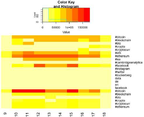
Fig.3. Heat map analysis
Dimensions
Fig.4. Scree plot
Hashtags and color key
#Ethereum - Blue
#Facebook - Green
#Bitcoin - Red
#zuckerM6g::::faceb00k
-
#lco e8^^^ #blockcfl6ln Sblockchalnl #ethereu^ypt°*yrr1 .№ Sbltcolnl ^greum #bltcoln17
Scryptol #eth-fitter
10 en t sole
-
11 ' #cryptocurr
9 16*
Dimension 1. X = 0.119. 1=31%
Fig.5. Factor Score (Asymmetric plot)
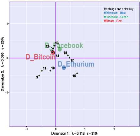
Fig.6. Factor Score (Symmetric plot)
-0.4 0.0 0.4
Contributions
Fig.7. Most Contributing Variables
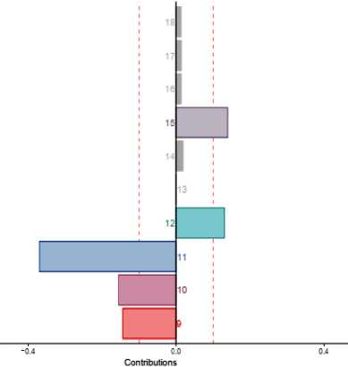
Fig.8. Contribution of all weeks
Find the topics associated with the term “market”
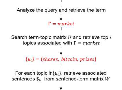
(u1) = {Shares} ^ {Sentences$h } (u2) = (bitcoin} ^ {Sentences$h} (u3) = (prizes) ^ {Sentences$h}
For each sentence in ($h) , retrieve associated topics (uk} from sentence-topic matrix 0
{ uii,ui2,uuj { U11,U12,U1(,}
{uh1,uh2,uh I ,}
Return the retrieved topics
Fig.9. Query evaluation scenario for topic extraction
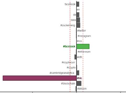
31% and 25% of total inertia has been explained by dimensions 1 and 2 respectively. More the data points are away from the center, more the inertia (variance) they possess. If distance between data points is more, then they carry good pattern among themselves. For example, #cambridgeanalytica has been discussed more in weeks 12 and 15 under hashtag #facebook. So, this visualization gives notion of information and patterns among data points. In order to check whether variables associated with data points really possess good information, the plot of most contributing variables in depicted in figure 7.
Variable associated with #cryptocurr (shown in blue color) under #facebook category and #crypto (shown in red color) under #bitcoin are the most contributing variables.
Figure 8 shows the plot of weeks according to their contribution for topics being discussed in respective week. Weeks 9, 10, 11, 12, and 15 are important. It shows something happened in News during these weeks that caused the words closer to these weeks behave similarly.
C. Results Discussion
After performing EDA and CA, we applied our proposed approach – online latent semantic indexing constrained by regularization on Twitter data. Tweets are associated with the hashtags #bitcoin, #ethereum, and #facebook. Table 9 shows the top 5 topics extracted in each week from 9 to 18 for the hashtags #bitcoin, #ethereum, and #facebook.
Figure 9 shows the query evaluation scenario when user sends query to get the topics associated with a given term. Let us say, uses sends a query: Find the topics associated with the term “market”. Initially, the query is analyzed and terms directly mentioned in query are retrieved. Therefore, for the given example, the termtopic matrix ‘U’ is searched and top i topics associated are retrieved, i.e. top topics
{shares , b it co in, and prizes] are retrieved. For each topic, retrieve the sentences from sentence-term matrix ‘W’ assuming each topic as a term. For each sentence, choose topics {u fc } from sentence-topic matrix ‘O’ , and return retrieved topics. These topics are the topics related to the term Г = market. The extracted topics are given as
^11, ^12, ■" , U1Z
^21, ^22, ■" , ^21
U31 , U32 , ■" , U3Z
With the help of both sentence-term matrix ‘W’ and sentence-topic matrix ‘O’ , the approach also performs extraction of topics implicitly present.
Table 9. Top 5 topics extracted using proposed approach for each week from 9 to 18
(a) Topics extracted with #bitcoin
|
Week 9 |
Week 10 |
Week 11 |
Week 12 |
Week 13 |
Week 14 |
Week 15 |
Week 16 |
Week 17 |
Week 18 |
|
Dominance |
Market |
croatia |
recent |
market |
bitcoin |
destroy |
supporters |
Lacklustre |
Blockchain |
|
project |
Change |
Bitcoin |
audit |
Bounce |
scammers |
value |
Contactez |
Markets |
Telephone |
|
CRYPTO |
Masterminds |
rank |
payment |
water |
account |
Crypto |
reward |
Bitcoin |
Electron |
|
successs |
Bitcoin |
Space |
sagolsun |
Analysis |
news |
Madness |
Hublot |
Cash |
future |
|
investors |
Ripple |
quality |
cryptocurrency |
Dogecoin |
livestramers |
podcast |
decentralisedsystem |
crypto |
investment |
|
Altcoin |
CryptoCashbackRebate |
pembeli |
BitLicense |
Support |
akan |
Transtoken |
cash |
trading |
History |
(b) Topics extracted with #facebook
|
Week 9 |
Week 10 |
Week 11 |
Week 12 |
Week 13 |
Week 14 |
Week 15 |
Week 16 |
Week 17 |
Week 18 |
|
download |
Clarification |
|
Shkreli |
deactivated |
Censoring |
fight |
Cryptocorner |
Unbearably |
technologies |
|
Hype |
guide |
failed |
Brotheers |
Optimization |
virus |
content |
Market |
Snapchat |
Market |
|
|
teenager |
edumacated |
Zuckerberg |
socialmedia |
catie |
brother |
drop |
video |
fund |
|
archive |
Business |
broadcasting |
friend |
Regulating |
Scanning |
privacy |
|
lol |
suspend |
|
Retargeting |
uploaded |
live |
million |
Cryptocurrency |
Messenger |
graduation |
friday |
data |
Stock |
(c) Topics extracted with #ethereum
|
Week 9 |
Week 10 |
Week 11 |
Week 12 |
Week 13 |
Week 14 |
Week 15 |
Week 16 |
Week 17 |
Week 18 |
|
Altcoin |
CryptoCashbackRebate |
pembeli |
BitLicense |
Support |
akan |
Transtoken |
cash |
trading |
History |
|
airdropping |
Kapsus |
Cryptocurrency |
terjual |
VertChain |
wallet |
free |
future |
Darico |
currency |
|
hedgefund |
Localcoin |
Food |
crypto |
Airdrop |
cryptocurrency |
market |
RAXOM |
crypto |
Binance |
|
Limited |
Bitcoin |
Ico |
price |
happy |
sidechain |
Casper |
airdrop |
Ethereum |
Bitcoin |
|
investment |
price |
Blockchain |
drop |
shopping |
beacon |
revolutionary |
Truffle |
Mining |
Exchange |
V. Conclusion
We have proposed a deep learning model for explicit and implicit detection of dynamically generated topics from streaming data by online version of Latent Semantic Indexing constrained by regularization. The approach mentioned is scalable to large dataset. It is flexible to support both long normal text and short text for modeling the topics. The model is adaptive such that it is updated incrementally and performs temporal topic modeling to get notion of evolution and trends of topics over time. Topic modeling approach supports extraction of implicit and explicit topics from sentences also. This model can be treated as first step towards implicit and explicit aspect detection for aspect based sentiment analysis on social media data.
We have performed exploratory data analysis and correspondence analysis on real world Twitter dataset. Results state that our approach works well to extract topics associated with a given hashtag. Given the query, the approach is able to extract both implicit and explicit topics associated with the terms mentioned in the query. The next step would be to perform the performance analysis with reference to standard performance metrics.
References Adaptive model for dynamic and temporal topic modeling from big data using deep learning architecture
- A. R. Pathak, M. Pandey, and S. Rautaray, “Construing the big data based on taxonomy, analytics and approaches,” Iran J. Comput. Sci., vol. 1, no. 4, pp. 237–259, Dec. 2018.
- D. M. Blei, “Probabilistic Topic Models,” Commun. ACM, vol. 55, no. 4, pp. 77–84, Apr. 2012.
- D. M. Blei, A. Y. Ng, and M. I. Jordan, “Latent dirichlet allocation,” J. Mach. Learn. Res., vol. 3, no. Jan, pp. 993–1022, 2003.
- T. Hofmann, “Probabilistic latent semantic analysis,” in Proceedings of the Fifteenth conference on Uncertainty in artificial intelligence, 1999, pp. 289–296.
- S. Deerwester, S. T. Dumais, G. W. Furnas, T. K. Landauer, and R. Harshman, “Indexing by latent semantic analysis,” J. Am. Soc. Inf. Sci., vol. 41, no. 6, pp. 391–407, 1990.
- X. Cheng, X. Yan, Y. Lan, and J. Guo, “Btm: Topic modeling over short texts,” IEEE Trans. Knowl. Data Eng., no. 1, p. 1, 2014.
- Y. Zuo, J. Zhao, and K. Xu, “Word network topic model: a simple but general solution for short and imbalanced texts,” Knowl. Inf. Syst., vol. 48, no. 2, pp. 379–398, Aug. 2016.
- K. Nigam, A. K. Mccallum, S. Thrun, and T. Mitchell, “Text Classification from Labeled and Unlabeled Documents using EM,” Mach. Learn., vol. 39, no. 2, pp. 103–134, May 2000.
- P. Xie and E. P. Xing, “Integrating document clustering and topic modeling,” arXiv Prepr. arXiv1309.6874, 2013.
- D. M. Blei, J. D. Lafferty, and others, “A correlated topic model of science,” Ann. Appl. Stat., vol. 1, no. 1, pp. 17–35, 2007.
- M. Hoffman, F. R. Bach, and D. M. Blei, “Online learning for latent dirichlet allocation,” in advances in neural information processing systems, 2010, pp. 856–864.
- Q. Wang, J. Xu, H. Li, and N. Craswell, “Regularized latent semantic indexing,” in Proceedings of the 34th international ACM SIGIR conference on Research and development in Information Retrieval, 2011, pp. 685–694.
- L. AlSumait, D. Barbará, and C. Domeniconi, “On-line lda: Adaptive topic models for mining text streams with applications to topic detection and tracking,” in Data Mining, 2008. ICDM’08. Eighth IEEE International Conference on, 2008, pp. 3–12.
- Y. Wang, E. Agichtein, and M. Benzi, “TM-LDA: efficient online modeling of latent topic transitions in social media,” in Proceedings of the 18th ACM SIGKDD international conference on Knowledge discovery and data mining, 2012, pp. 123–131.
- X. Li, A. Zhang, C. Li, J. Ouyang, and Y. Cai, “Exploring coherent topics by topic modeling with term weighting,” Inf. Process. Manag., 2018.
- K. D. Kuhn, “Using structural topic modeling to identify latent topics and trends in aviation incident reports,” Transp. Res. Part C Emerg. Technol., vol. 87, pp. 105–122, 2018.
- S. Brody and N. Elhadad, “An Unsupervised Aspect-sentiment Model for Online Reviews,” in Human Language Technologies: The 2010 Annual Conference of the North American Chapter of the Association for Computational Linguistics, 2010, pp. 804–812.
- A. R. Pathak, M. Pandey, S. Rautaray, and K. Pawar, “Assessment of Object Detection Using Deep Convolutional Neural Networks,” in Intelligent Computing and Information and Communication, 2018, pp. 457–466.
- A. R. Pathak, M. Pandey, and S. Rautaray, “Deep Learning Approaches for Detecting Objects from Images: A Review,” in Progress in Computing, Analytics and Networking, 2018, pp. 491–499.
- A. R. Pathak, M. Pandey, and S. Rautaray, “Application of Deep Learning for Object Detection,” Procedia Comput. Sci., vol. 132, pp. 1706–1717, 2018.
- A. B. Dieng, C. Wang, J. Gao, and J. Paisley, “Topicrnn: A recurrent neural network with long-range semantic dependency,” arXiv Prepr. arXiv1611.01702, 2016.
- Y. Li, T. Liu, J. Hu, and J. Jiang, “Topical Co-Attention Networks for hashtag recommendation on microblogs,” Neurocomputing, vol. 331, pp. 356–365, 2019
- P. Gupta, F. Buettner, and H. Schütze, “Document informed neural autoregressive topic models,” arXiv Prepr. arXiv1808.03793, 2018
- K. Giannakopoulos and L. Chen, “Incremental and Adaptive Topic Detection over Social Media,” in International Conference on Database Systems for Advanced Applications, 2018, pp. 460–473
- Y. Zhang et al., “Does deep learning help topic extraction? A kernel k-means clustering method with word embedding,” J. Informetr., vol. 12, no. 4, pp. 1099–1117, 2018
- W. Gao, M. Peng, H. Wang, Y. Zhang, Q. Xie, and G. Tian, “Incorporating word embeddings into topic modeling of short text,” Knowl. Inf. Syst., pp. 1–23, 2018
- X. Li, Y. Wang, A. Zhang, C. Li, J. Chi, and J. Ouyang, “Filtering out the noise in short text topic modeling,” Inf. Sci. (Ny)., vol. 456, pp. 83–96, 2018
- H. Zhang, B. Chen, D. Guo, and M. Zhou, “WHAI: Weibull Hybrid Autoencoding Inference for Deep Topic Modeling,” in International Conference on Learning Representations, 2018
- H. Abdi and L. J. Williams, “Principal component analysis,” Wiley Interdiscip. Rev. Comput. Stat., vol. 2, no. 4, pp. 433–459, 2010.
- H. Abdi, “Multivariate analysis,” Encycl. Res. methods Soc. Sci. Thousand Oaks Sage, pp. 699–702, 2003.
- H. Abdi and L. J. Williams, “Correspondence analysis,” Neil Salkind (Ed.), Encyclopedia of Research Design. Thousand Oaks, CA: Sage. 2010.
