Adaptive RBFNN strategy for fault tolerant control: application to DSIM under broken rotor bars fault

Author: Noureddine Layadi, Samir Zeghlache, Ali Djerioui, Hemza Mekki, Fouad Berrabah
Journal: International Journal of Intelligent Systems and Applications @ijisa
Article in issue: 2 vol.11, 2019.
Free access
This paper presents a fault tolerant control (FTC) based on Radial Base Function Neural Network (RBFNN) using an adaptive control law for double star induction machine (DSIM) under broken rotor bars (BRB) fault in a squirrel-cage in order to improve its reliability and availability. The proposed FTC is designed to compensate for the default effect by maintaining acceptable performance in case of BRB. The sufficient condition for the stability of the closed-loop system in faulty operation is analyzed and verified using Lyapunov theory. To proof the performance and effectiveness of the proposed FTC, a comparative study within sliding mode control (SMC) is carried out. Obtained results show that the proposed FTC has a better robustness against the BRB fault.
Double star induction machine, Radial base function neural network, Sliding mode control, Robustness, Fault tolerant control, Broken rotor bars
Short address: https://sciup.org/15016572
IDR: 15016572 | DOI: 10.5815/ijisa.2019.02.06
Text of the scientific article Adaptive RBFNN strategy for fault tolerant control: application to DSIM under broken rotor bars fault
Published Online February 2019 in MECS
The double star induction machine (DSIM) belongs to the category of multiphase induction machines (MIM). It has been selected as the best choice because of its many advantages over its three-phase counterpart. The DSIM has been proposed for different fields of industry that need high power such as electric hybrid vehicles, locomotive traction, ship propulsion and many other applications where the safety condition is required such as aerospace and offshore wind energy systems. DISM not only guarantees a decrease of rotor harmonics currents and torque pulsations but it also has many other advantages such as: reliability, power segmentation and higher efficiency. DSIM has a greater fault tolerance; it can continue to operate and maintain rotating flux even with open-phase faults thanks to the greater number of degrees of freedom that it owns compared to the three-phase machines [1-3].
The motors installed in the industry are 85% of squirrel cage motors [4]. Induction motors are subject to various faults; about 40% to 50% are bearing faults, 5% to 10% are severe rotor faults, and 30% to 40% are stator-related faults [5]. Broken bars has proved dangerous and may be the cause of other faults in the stator and the rotor itself because a broken rotor bar considerably increases the currents flowing in the neighboring bars, which causes the increase of the mechanical stresses (constraints) and consequently causes the rupture of the corresponding bars [6]. BRB fault can be caused by failures in the rotor fabrication process, overloads (mechanical stress), mechanical cracks or thermal stress [7].
-
II. Related Works
The main advantage of neural networks (NNs) is their capacity to approximate uncertainties in model-uncertain systems with complex and unknown functions without the need for precise knowledge of model parameters [8]. Several works based on NN controllers with an adaptive control technique have been proposed; [9] presents an adaptive neural network saturated control for MDF continuous hot pressing hydraulic system with uncertainties, the RBFNN-based reconstruction law is introduced to approximate the composite term consisting of an unknown function, disturbances, and a saturation error. In [10], a robust adaptive fault-tolerant control has been proposed for over-actuated systems in the simultaneous presence of matched disturbances, unmodeled dynamics and unknown non-linearity of the actuator, authors used the radial basis function neural network in order to have an approximation of the unmodeled dynamics. [11] proposes an actuator fault tolerant control using an adaptive RBFNN fuzzy sliding mode controller for coaxial octorotor UAV, simulation results show that, despite the rotor failure, the octorotor can remain in flight and can perfectly perform trajectory control in x, y and z and can also control yaw, roll and pitch angles. Inspired by [8], this paper proposes an adaptive RBFNN control method for a class of unknown multiple-input-multiple-output (MIMO) nonlinear systems with bounded external and internal disturbances (DSIM with defective rotor) in order to compensate the fault effect after estimating uncertainties. The proposed FTC is tested in healthy and defective conditions with other control methods applied on six-phase induction machine [12, 13]. The performance of these controllers is investigated and compared in terms of reference tracking of the rotor speed, the electromagnetic torque and the rotor flux. This paper has made several contributions in relation to recent research concerning the FTC:
-
• An intelligent FTC to properly control the torque, flux and speed tracking of a DSIM with a BRB defect has been proposed in this contribution, the application of the adaptive control RBFNN as FTC for DSIM in a faulty case is performed for the first time.
-
• Compared to [14, 15], the authors used non-linear observers for the detection and reconstruction of defects. In this article, the RBFNN is used to detect and reconstruct the faults.
-
• The proposed scheme could be interesting and this approach can achieve a tolerance to a wide class of system failures.
-
• Compared to [16], a multi three-phase induction motor drive is processed; the proposed FTC does not need a predictive model for fault tolerance.
-
• Compared to the passive fault tolerant control developed in [17], this paper proposes an adequate adaptive parameter-tuning law to overcome system disturbances and BRB faults without information of their upper bounds.
-
• Compared to the intelligent control presented in [18], the adaptive control law has been applied to all stages, increasing the controller's tolerance. In addition, the proposed FTC was dealing with a faulty machine while [18] was handling a healthy doubly-fed induction motor (DFIM).
-
• Compared with [19, 20], where the authors
respectively present a FTC of six-phase induction motor under open-circuit fault and a FTC of five-phase induction machine under open gate transistor faults, the degree of severity of the fault dealt with in this paper is more important since open phase fault tolerance is a specific feature of multiphase machines due to the high number of phases.
The remainder of this paper is organized as follows; the following section describes the DSIM faulty model. The design of the proposed FTC is carried out in section 4. Simulation results and their discussions are given in section 5. The last section is reserved for conclusion.
-
III. DSIM Faulty Model
In order to establish a faulty model of DSIM, we consider the rotor as a balanced three-phase system; the squirrel cage rotor is replaced by an equivalent three phase windings (single star winding) with equivalent resistance R and leakage L . When the rotor of the DSIM is broken, the rotor resistance is different than the nominal value [21], to simulate a BRB in the double star induction machine; we increase the resistance of a rotor phase by adding a defective resistance e . The first-order differential equations of the rotor voltages in the natural “ abc ” reference frame are given by:
abc abc d abc
Vr J-LRr J[Ir J + —[Ф r J dt
With:
L R r J -
■ R r
_ 0
L J - L v ,
[ Ф Г J - L ^ ra L i rb J - L / ra
Rr0
0 R r _
^rb ^rc J T b r,J JT vrb vc J T
Where:
[ Rr ] is the matrix of resistances, [ Ф abc ] is the flux vector, [ Iabc ] is the vector of currents and [ V°bc ] is the vector of tensions. When the BRB fault occurs, the resistances matrix becomes the following:
[ d 1 "
— Q - — p dt J
dt
d tt Ф, -
2 Lm
L + L mr
r
- R ,
L , + L m
Ф г
+
Ф , ( isq 1 + i sq 2 ) - PT L
L m R r
L , + L m
- Kf Q
( i sd 1 + i sd 2 ) + Г 1
|
"R, |
0 |
0 1 |
||
|
[ r Brb ] - |
0 |
R r |
0 |
(3) |
|
_ 0 |
0 |
R , + e _ |
d 1 isd 1 r { v sd 1
dt Ls 1
d 1
dtisq 1 L $1 { v2 1
-
R s 1 i sd 1 + ® s ( L s 1 i sq 1 + T M® gl )} + Г 2
-
R s 1 i sq 1 - ® s ( L s 1 i sd 1 + ф г ) } + Г 3
In this case, the voltages equation in (1) becomes:
5 .
d 1
— iso 1 - —( v so 1 - R s 1 i so 1 )
dt L s 1
abc BRB abc d abc
V , ] - [ R r ][ I , ]+-;;[ ф r ]
dt
By applying the park transformation that conserves the energy on (4), we obtain the equation of the tensions in the ( d - q ) reference frame:
[i;- ] - [p, (9)][r7 ][p, (Ж1 [id40 ]+- [ф , ]+ dt
[ P r 9 - { [ р ( У ) ] - 1 } [ф d qo ] (5)
Where:
[ Vrdqo ] - [ vrd vrq v o L is the voltages vector,
[ I-'1 ] - [ ird irq iro ] T is the currents vector and [ Ф ,"" ] - [ ф г- Ф , Ф го ] T is the rotor flux vector. [ P r ( 9 ) ] is the transformation matrix of the rotor winding, is given by:
[ P , 9 )1- 21
P
P
P
With:
j/V2 1/V2
1/V2J
P 11 - cos ( 9 s - 9 , ) ; P 12 - cos ( 9 s - 9 , -
")
P13 - cos (9s - 9,
2 n
■) ; P 21 - — sin ( 9 s - 9 , )
P 2 - - sin
in (9 - 9,
- 2 П ) ; P 23 -- sin ( 9 s - 9 ,
2 П
+т)
/
d
® , ^; dt
d
<9, s dt
Finally, The DSIM model in the presence of BRB faults is given by the following equations:
d 1
i sd 2 r { v sd 2
dt L d1
dt sq 2 2 Ln { v q q
-
R s 2 i sd 2 + ® s ( L s 2 i sq 2 + TM ® gl )} + Г 4
-
R s 2 i sq 2 - ® s ( L s 2 i sd 2 + ф г ) } + Г 5
d 1
— z i = — (v л — R J ,)
so 2 so 2 s 2 so 2
dt Ls 2
Where:
Г i - 1,5 represent the fault terms due to a broken bar fault, they are given by:
Where:
Г
—
R r
a
® gi 1
Ф - + . L , + L m в ( L , + L m ) в J Г
a L m
RL
в L + L L + L rm rm
( i sd 1 + i sd 2 )
Г 2 -
<
Г 3 -
—
Ю s Ю gl Ф г
Ls 2
L 7 — ^Юф
L s 2
1 I Lr I
Г 4 - —I-- T r I ® s ® gl Ф г
L s 2 V n )
Г 5
—
a -
L
,--МФ.ф,
L s 2 7
aa a2 + (a3 — )( a5
a 2
—
a 3 a 4 a 2
aa aa
( a 6 - —)- —
a 2
a 2
a 5I a в - a4 +
-
a, 1
-
2 a 2 1 a
—
a 4 a 3
—
a 2 aa
a 2
Y -
a6a 2 - 2 a2a3a 5 + a4a 32 + axa 2 - axa^a6 2
- a 3 + axa6
a6a 2 - 2 a2a3a 5 + a4a 32 + axa 2 - aa4a6 a2a 3 - axa5
Where:
f 2 =
p
- Rr
—
K
-f Q
a 2 ( a6a 2 - 2 a3a 5) + a4a 32 + ax ( a 2 - a4a 6) a2a 6 - a3as
e e _ _ „ a, = - + rr — cos(26 - 26)--- sin(26 - 26)
13 6 r s 6 r s
a 2
a =
- cos(2 6 - 26, + - ) 3 rs 6
--e cos( 6 - 6 + - ) 3 rs 3
ee3
a 4 = + rr + cos(2 6 - 2 6 ) +-- - sin(2 6 - 2 6 )
43 6 r s 6 rs
-
V2
-
a. =-- e cos( 6 - 6 +— )
e
-
a, = + rr
IV. The Proposed FTC Design for Dsim
The goal is to design a FTC based on the RBFNN scheme for an uncertain DSIM model in the presence of BRB faults to properly handle the flux and speed tracking. The role of RBFNN systems is to approach the local nonlinearities of each subsystem by adaptive laws that respect the stability and convergence of the Lyapunov theory until the desired tracking performance is achieved. To design the proposed control, we operate with the defective DSIM model developed in (8), in the presence of BRB faults, so we have:
|
f d n Q dt |
= p m ф ( i ,+ i 2) + f r sq 1 sq 2 1 J L m + L r |
|
d |
LR |
|
It Ф ' |
- , J ( i sd 1 + i sd 2 ) + f 2 L r + L m |
|
d_. |
1 |
|
dtZsd 1 |
- -,-v sd 1 + f 3 Ls 1 |
|
d . |
1 |
|
dti sq 1 |
- —v sq 1 + f f |
|
Ls 1 (13) |
|
|
‘ d . |
1 |
|
dit1 so 1 |
- — vso 1 + f 5 Ls 1 |
|
d . |
1 |
|
dY s 2 |
- —v sd 2 + f , Ls 2 |
|
d . |
1 |
|
dtZ s q 2 |
- -J-v sq 2 + f 7 Ls 2 |
|
d . |
1 |
|
. dTY0 o |
- у v so 2 + f 8 Ls 2 |
Where:
L r + L m
Фг + Г1
f- - R L ;
f 3 T lsd 1
Ls 1
f = - R 1- /
J 4 T i sq 1
Ls 1
r - R1 • f5 = -i— iso 1
Ls 1
+ ® s i sq 1
—
f - -R2- f 6 T Lsd 2
Ls 2
f = - R 2. /
J 7 T i sq 2
L s 2
- Rs 2
f 8 L s 2 iso 2
+
® s i sd 1
® s T r T r ® gl
Ls 1
- ^ s ^ +Г
+ ® s i sq 2
—
+
® s i sd 2
+ Г
Ls 1
®T^®gi
Ls 2
+ Г 4
- ^ s ^ +Г
L s 2
RBF neural networks are used adaptively to approximate the unknown f ( i = 1,8 ) . The structures of RBFNN with receptive field units are shown in Fig.1. The radial-basis function vector H that indicates the output of the hidden layer is given by [8]:
H il = exP
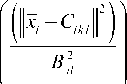
, ( i = 1,8 )
Where: x are the inputs state of the network, k is the input number of the network, l is the number of hidden layer nodes in the network, C and B represent the center of the receptive field and the width of the Gaussian function respectively. Hz = [ HiX Hi2 ... Hzn ] T with i = 1,8 are the output of the Gaussian function.
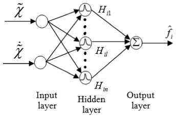
Fig.1. The structure of RBFNN
у = Гд со i ,, z , I л г i , i Д
-
х ^Y r r^r sd 1 sq 1 so 1 sd 2 sq 2 so 2 J
T = \_Фг to r i sd 1 isq 1 i so 1 i sd 2 i sq 2 i so 2 J (16)
i = { 1,2,3,4,5,6,7,8 }
The nonlinear functions f (xt) , i = 1,8 can be estimated by the RBFNN as follows:
f ( x ) = W T H( x) , i = 1,8 (17)
Where: x is the input vector, W are the weights vector parameters of the adjusted neural network and H z ( x ) are the outputs of the Gaussian function. Let us define the actual functions f ( x ) :
f (x ) = W * TH (x) + to( x), i = 1,8(18)
Where: W * are called the optimal parameters used only for analytical purposes and to ( x ) are the approximation errors, such as:
I to(x)|< ^
Where:
to ( x ) are unknown positive parameters.
The parametric errors are given by:
W = W -W* , i = 1,...,8(20)
In order to achieve precise flux and speed tracking, some assumptions have been put:
Assumption! The functions f (x) , i = 1,8 are continuous nonlinear functions assumed to be unknown.
Assumption2. The reference signals Q * , Ф* , i *dl , i * x , i * , i * , i * , i * and theirs first derivatives are bounded sd 2 sq 2 so 1 so 2
and continuous.
Assumption3. The rotor and stator currents and the rotor speed are available for measurement.
The tracking errors and their filtered errors are given by:
-
• For rotor speed
Q(t) = Q(t)-Q*, Sn = Q(t) + A£Q(t)dT , with Q(0) = 0(21)
For rotor flux
Фг (t) = Фг (t) - Ф**, S^ = Фг (t) + A £ Фг(r) dT, with Ф (0) = 0(22)
-
• For stator currents
i'sd1 (t) = isd 1 (t) - C 1 , Sisd 1 = isd 1 (t) + ^isd 1 £ isd 1 (T) dT with isd 1 (0) = 0(23)
isd 2 (t) = isd 2 (t) — isd 2 , Sisd 2 = isd 2 (t) + ^isd 2 isd 2 (t) d T with isd 2 (0) = 0(24)
isq! (t) = isq 1 (t) — iq 1 , Sisq1 = isq1 (t) + ^isq1 isq1 (t) dT with isq1 (0) = 0(25)
isq 2 (t) = isq 2 (t) — i* 2 , S.sq 2 = isq 2 (t) + ^isq 2 £ isq 2 (T) d T with isd2 (0) = 0(26)
-
• For homopolar components
iso1 (t) = iso1 (t) - i*o1 , Siso1 = iso1 (t) + ^iso1 £ iso1 (T) dT with io1 (0) = 0(27)
iso 2 (t) = iso 2 (t) — iso 2 , Siso 2 = iso 2 (t) + ^iso 2 -so 2 (t) dT with iso2 (0) = 0(28)
Where:
^ Q , A p r , ^ isd 1 , ^ isd 2 , ^ isq 1 , ^ isq 2 , ^ iso1 and ^ iso 2 are strictly positive design parameters, and we admit that:
|
i sq 1 |
+ Z э sq 2 |
i sq ; * |
i sd 1 + i sd 2 = i sd |
|
|
* i4q 1 |
* = i sq 2 |
i sq 2; |
* * * isd i sd 1 i sd 2 2 |
(29) |
|
i * i so 1 |
= 0; |
* i о = so 2 |
0 |
The following adaptive fuzzy control laws are made in the case where the dynamics of DSIM is uncertain:
* i sq
J ( L m + - r ) — WH 1 ( X ) — k 11 - n — Vanh | S P L m V r V V S iq
*
isd =
- + L t .
-r--^ |— W 2 T H 2 ( X 2 ) — k 21 - фг
L m R r V
—
1 t h Г S ^ k 22 tanh | ----
V S sd.
v sd 1 = -s 1 C W3 TH 3 ( X 3 1 k 31 Sisd 1 — k 32 tanh C S isd 1
V V S sd 1,
<
c Г -..„, vsq 1 = -s 1 | —W4 H4 (X4 ) — k41 Sisq 1 — k42 tanh | ----
V V S sq 1,
V. 1 = — W 5 T H 5 ( x ) — k 51 S iso 1 — k 52 tanh | —
V S iso 1 -
v sd 2 = Ls 2 | W 6 H 6 ( x 6 ) k 61 Sisd 2
—
k 62 tanh | -<^
V S isd 2
r r -_;
v sq 2 = Ls 2 | W7 H 7 ( x 7 ) k 71 Sisq 1 k 72 tanh |
V V S isq 2 ,
-
k 12 = — ^ kx Y k 1 k 12 + Y k 1 S n tanh | -^ I
V S isq J
Г - , .)
-
k 22 = — ^ k 2 Y k 2 k 22 + Y k 2 S ^ r tanh | ---- I
V S isd J
-
k 32 = — ^ k3 Y k3 k 32 + Y k3 S isd 1 tanh | S isd 1 1
-
3 3 3 V S .sd 1 J
r S„„ ,3
-
k 42 = — ^ k 4 Y k 4 k 42 + Y k 4 S isq 1 tanh | ----- I
V S isq 1 J (32)
-
k 52 = — ^ k 5 Y k 5 k 52 + Y k 5 S iso 1 tanh | S iso 1 1
-
V S iso1 J r -^ k^0 = — < 7, y k.^ + y -,^ э tanh — isd 2 62 k 6 k 6 62 k 6 isd 2
-
V S isd 2 J
-
k 72 = — 7 k 7 Y k 7 k 72 + Y k 7 S isq 2 tanh | S isq 2 |
V S isq 2 J
Г - _,3
-
k 82 = — 7 k 8 Y k 8 k 82 + Y k 8 S iso 2 tanh | ----- I
V S iso 2 J
v so 2 = W 8 H 8 ( X 8 ) k 81 S iso 2
—
S k tanh iso 2 82
V S iso г.
The design parameters k remain constants for i = 1,8 . Ssq , Ssd , S sd 1 , Ssq 1 , S so 1 , S sd 2 , Ssq 2 and S so 2
are absolutely positive design constants, usually are small. tanh (.) is the abbreviation hyperbolic tangent function. Now, according to [18], to estimate the unknown neuronal network weights ( W * ) and the unknown parameters ( k * ) for i = 1,8 , we adopt the following adaptive laws :
-
• For W :
-
W 1 7 w 1 Y w 1 W + Y w 1 S n H 1 ( x 1 )
W =— 7 Y W W 2 + Y W S^H 2 ( X 2 )
-
W3 = — ^W3 YW3 W3 + YW3 Sisd 1 H3
W4 =— 7W YW4 W4 + YW4 Sisq 1 H4
-
W 5 = — 7 W5 Y W5 W 5 + Y W 5 S iso 1 H 5 ( X 5 )
W6 =— ^W6 Yw6 W6 + Yw6 Sisd 2 H6
-
W7 = — ^W7 YW7 W7 + YW7 Sisq 2 H7
W B = — ^ W 8 Y W 8 W 8 + Y W8 S iso 2 H 8 ( X 8 )
Where:
7t , Yt , Yt , 7, > 0 (For i = 1,8 ); these parameters are design constants.
-
Theorem 1
The following properties are valid for DSIM modeled by (8) and controlled by the adaptive laws presented in (31) and (32):
-
• The signals delimitation is guaranteed in closed-loop.
-
• The optimal choice of the setting parameters ensures the exponential convergence of the errors variables n ( t ) , Ф г ( t ) , i sd 1 ( t ) , i sq 1 ( t ) , i sd 2 ( t ) , i sq 2 ( t ) , i so 1 ( t ) and i so 2 ( t ) to a ball With an insignificant radius.
The proof of Theorem 1 is based on Lyapunov's theory of stability. It is presented by a feedback structure with two consecutive steps:
Step 1: The purpose of this step is to lead the speed to its desired reference by an adequate speed controller. Using the formula of the filtered rotor speed error defined in (21):
Sn =n ( t ) + Xn j' 6 ( r ) d T (33)
• For k *
Using (13), the time derivative of S is:
SQ = Q (t ) + Лп Q (34)
S Q = p,А,Фг^ 1 + i q 2 ) + f -Q * + ^ q Q (35) J L m + L r
S Q = h l ( x 1 ) + p- , Lm т Ф г 4q (36)
J Lm + L
Where:
h ( x ) = f -Q * + Xa Q and i * is the reference value of ( isq i + isq 2 ) that regulates the rotor speed and ensures the capacity of the load disturbances rejection. The Lyapunov function associated with the rotor speed error is presented by:
-
V - = - S2
The time derivative of (37) is:
-
V1 = SQ h- (x-) + SQ p2 -Lm- PriSq(38)
J Lm + Lr
The following adaptive fuzzy system is developed to approximate the uncertain continuous function h ( x ):
hl (x-) = W-TH- (x-)
h-(x- ) = W-TH (x-) + ®i (x-)
-
h- (x-) == -W-TH- (x-) + W-TH- (x-) + to- (x-)
Where: W = W - W * is the parameter error vector. By replacing (41) in (38), we obtain:
-
V - = - S Q W -T H - ( x - ) + S Q W h ( x - ) +
SQ to- (x-) + SQ p2 -Lm- Ф^(42)
J L m + L r
Where: to is an unknown constant such as:
| to- (x- )|< to-(43)
By choosing the expression of i * presented in (30) and using (43), we can make the following inequality:
-
V - <- s Q W - H - ( x - ) + k*X 2 S q|-
- ( sA
knSn tanh -2- - k„S2
" V£isq)
Where:
k;2 = ^(45)
Lemma 1 the set { ^ > 0, x e ^ } check the following inequality [18]:
-
0 < И - x tanh | — | < ^ = p^
-
< I £.)(46)
, p = e"<1+p ) - 0.2785
By exploiting (46), (44) becomes:
-
V - <- S Q W - H - ( x - ) + k*n e sq -
- ~(sA .
kuSn tanh -^ - kuS^(47)
“ I£.q )
Where:
k-2 = k-2
8 =Q.T1%5 8.
( isq isq
The Lyapunov function linked to the adaptive laws that estimate the unknown parameters W * and k * is defined by:
V = V +---WTW +---k. 2
2 1 1 112
2/W
The dynamics of Lyapunov function verify the following inequality:
V 2 < - S Q W -T H - ( x - ) + k -*2 e sq - k -2 S 2 tanh [ SA )-
V e isq /
-
k..S2 +---WTW +---k„A(50)
-
-- Q - - -2-2
2/6-
By substituting the values of W and k chosen in (31) and (32), respectively, V will be bounded by the following expression:
-
V2 < k*2esq -k--S2 -^W- WTW- -ak- k-2k-2(5-)
Property:
-
■-0 T 0 <- -^2 + - p*n2
[ 22
,0-0-0 ' G^ m
Where: m is a positive integer number. By using (52), (51) takes the following form:
V <-^11SQ --W;-7k2 + ^1(53)
With:
^1 = k* ^ + -H iWlf + -^ k*(54)
The stabilization of the filtered errors
S , S , S , S , S and S will be achieved in the isd1 isq1 iso1 isd2 isq2
following step.
Step 2: The aim of this step is to design the following control laws: is * d , vsd 1, vsq 1, vso 1, vsd 2, vsq 2 and vso 2 .The
Lyapunov function adapted to this step is given by:
V = V 2 + 2 S ? + 2 S d i + X S - i + 2 ^ +
1 S 2 + 1 S ^ 2 + 1 S 2 (55)
The dynamics of the Lyapunov function verify the following inequality:
V < - k. S 2 - ^W- II W l|2 - - k k 2 + X + SS +
3 11 Q HI 12 1 Ф Ф sw 1sm 1 + s 1 Sisq 1 + s s^ + s d 2 Sisd 2 +
S sS - । S. .,8 1(56)
sq2 sq2 so2
The derivatives of the filtered errors are obtained using (8) and (21) - (28):
LmRr•*
Ф L + L„ sq f 2 Ф Ф Ф г
S isd 1 T v sd 1 + f 3 + ^ isd 1 i sd 1 i isd 1
L s 1
1*
S isq 1 = T v sq 1 + J 4 + ^ isq 1 i sq 1 i isq 1
Ls 1
S iso 1 Г v so 1 + f 5 + ^ iso 1 i so 1 i iso 1
Ls 1
|
S isd 2 |
1 T vsd 2 + f 6 + ^ isd 2 i sd 2 Ls 2 |
* i isd 2 |
|
isq 2 |
1 T vsq 2 + f 7 + ^ isq 2 i sq 2 Ls 2 |
* i isq 2 |
|
iso 2 |
1 = ~ v o 2 + f 8 + Z iso 2 i so 2 - L s 2 |
i * so 2 |
V 3 <- k 11 S Q - -'л |W 1f - -" k 2+ 5 +
(, lr .* f, 1
S? I h2 (X 2 )+ , т isq I + Sisd 1I h3 (X3 )+ , vsd 1
x Lr Lm 7 x Ls 1
Sisq 11 h4 (X4 ) + X vsq 1 I + Siso 1 I h5 (X5 ) + Y" v.so1 I + x Ls 1 7 x Ls 1
Sisd 2 I h6 (x6 ) + 7^ vsd 2 I + S.sq 21 h7 (x7 ) + 7^ visq 2 I + x Ls 2 7 x Ls 2
Siso21 h8 (x8) + vso2 I x Ls 2
'Ssd = 0.2785Ssd |
Ssd 1 = 0.2785£z2d, |
Ssq 1 = 0-2785SKq 1 |
Siso 1 = 0.2785s. so 1 |
Ssd 2 = 0.2785s. sd 2 |
Sisq 2 = 0.2785Sisq 2 |
Ss„ 2 = 0.2785£zso 2 |
{W*, k*}, i = 2,8 are unknown parameters, their estimation requires an adaptive law defined by the following Lyapunov function:
Where:
; k;=д _ i = 2,8
V4 = V3 | +—W2TW2 2Yw2 2 2 | 12 +n k 22 2Yk2 | +—W3TW3 2Yw3 3 3 | + |
1k2 2Yk3 32 | + W4TWq 2yw4 | 12 + k 42 2Yk4 | +—W5TW5 2Yw5 5 5 | + |
1 k2 2Yk5 52 | 1 ~T ~ +---W^W, 66 2'wb | + k2 62 2Yk6 | +—W7TW7 2Yw, 7 7 | + |
121 -----k72+-- 2Yk 2Yw k7 W8 | - W8TW8+• | 12 82 2Yk8 | (69) |
The derivation of (69) gives:
By exploiting (46), the inequality (64) becomes:
V3 < - kn "2 - "1- ||Wl|2 - " k.2 + ?1 - ", WTH2 (X2) +
V4 < - k11 S2 - "W |Wif - " k2 + £1 - ", W^H2 (X2 ) +
k*2 Ssd - k22 ", tanh fy-1-k21 " - "sd 1 W H3 (X3) +
k32 Sisd 1 - k32 "zsd 1 | tanh | | hv h isd1 . Sisd 1 V | 1-k31 "sd 1 - "isq 1 W4TH, (X4 ) + |
k42 Sisq 1 - k42 "isq 1 | tanh | | "sq 1) S Sisq 1 V | - k41 "isq 1 - "so1 WTH5 (X5 ) + |
k52 Siso1 - k52 "iso 1 | tanh I | fSoL' V Siso1 V | 1-k51 S-o1 - "isd 2 WTH6 (X6 ) + |
k62 Sisd 2 - k62 "isd 2 | tanhI | "isd 2" S JO ) isd2 | 1- k61 "isd 2 - "isq 2 WTH7 (X7 ) + |
* 72 ^isq 2 ^72 ° isq 2 | tanh I | f "isq 2 V Sisq 2, | j-k71 "isq 2 - "iso 2 W8TH8 (X8 ) + |
k82 S2 -k82Siso2 tanhI — I-k81Sio2 (66)
V Siso 2 V
k2*2Ssd -k22", tanhf^-1-k21" -S . 1 W3H3 (X3) + k3*2 S,sd 1 -k32"sd 1 tanhI"isd11-k31 "isd 1 -"sq 1 WTH4 (X4) + V £isd 1 7
k*2Sisq 1 -k42"sq 1 tanhfSisq^|-k41 S2q 1 -"м W?H5 (X5) +
k*2 Sis01 - k52 "iso1 tanh | "iso11-k51 "iso1 - "sd 2 WT H6 (X6 ) + V Siso1 V k6*2 Ssd 2 - k62 "sd 2 tanh f "isd21-k61 "isd 2 - "isq 2 W7T H7 (X7 ) + Sisd 2
k*2 Sisq2 - k72 "isq2 tanhf"isq2 |-k71 "isq2 - "iso2 W8TH8 (X8) + V Sisq 2 V k82 Sso 2 - k82 "so 2 tanh f "iso21-k81 S^so 2 + Wj W2 +
V Siso 2 V 2Yw2
Where:
----k22 k22 +--W^ W^ +--k32 k32 +--^4 ^4 +
2Yk2 2Yw3
2Y3
Y
And:
'k.2 = k -k* _ i = 2,8
1 ~ - 1 ~T • k4 k42 + WTW5
^Yk4 2/w5
----k62k62 +----W7TW7
62 62 7 7
2Yk6 2Yw,
1 ~ • 1 ~T •
+ k52 k52 + W6TW6+
2Yk5
+----k72 k72 +----W8W„+
72 72 88
2Yk7 2Yw8
82 82.
2Y,
If we multiply (73) by the exponential term en , we obtain [18]:
By using (52), we obtain:
V4<-k„ SQ --^IWII2 -^^-k21S’ --6W2||2 -^k222 --k31 Sisd 1 --гWalP -^k322 -k41 Sisq 1 -
W4ir - ^ k2 - k51SL1 - ^ w/ - ^ k22 - k61SM2 - —IW||2 - —k622 - k71SL - —W ||2 -
61 isd2 6 62 71 isq27
—7"k722 -k81 Siso2W|W,||~k2 + £1 + £2 + £3+
^4 + £5 + £ + £7 + £(71)
Where:
£2 = k*2 £isd | +-W- И2 | + ^k^ k*22 222 | ||
£3 = k32 £isd 1 | +-^ гл2 | + —k3- к*г +2 k32 | ||
£4 = k42 £isq 1 | +-W- w;r | + -k4- ^‘2 +2 k42 | ||
( | * £5 ^52 £iso 1 | +-W" iw;iP | + ^ k k5 22 252 | (72) |
£6 = k62 £isd 2 | +^- w;r | + -k- k622 262 | ||
* £7 ^72 £isq 1 | +-^ W7I2 | + -- ky2 272 | ||
£8 = k82 £iso 2 | +^W- W‘lP | + -k- k81 282 | ||
A simplified form of (71) can be presented | as follows: | |||
V4 <-qV4 + A(73)
With:
A = £ + £ + £3 + £4 + £5 + £5 + £7 + £ n = min {2 k11,2 k21,2 k3,, 2 k41,2 k51>2 k61,2 k7, ,2 k81,
-e Yex,-e2 Ye,,-3 Y 63, —e^ Y64, -■ Ye,, -e6Ye6,
1 1(74)
- - Ye,,-e8Yes,nk}
n = min {-k1 Ykv, -k2 Yk2, -k3 Yk3, -k4 Yk4, -k5 Yk5,
_ -k6 Yk6,-k7 Yk7,-k8Yk,}
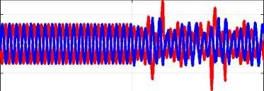
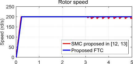
d(V en) dt The integration of (75) from 0 to t gives us: MT TO ---SMC proposed in [12, 13]---Proposed FTC| I I I I I 2 2.5 3 3.5 4 4.5 5 time (s) (b) time (s) (c) x E 0.5 Zoom of stator current | — SMC proposed in [12, 13] —Proposed FTC 3 time (s) (d) 3.5 Rotor flux — SMC proposed in [12, 13] --Proposed FTC time (s) (e) -50 L Electromagnetic torque — SMC proposed in [12, 13] ^—Proposed FTC HM 1 2 3 4 5 time (s) (f) Fig.2. Pre-fault (t <3s) and post-fault (t >3s) performance of SMC proposed in [12, 13] and proposed FTC for DSIM VI. Conclusion In this paper, an adaptive RBFNN control method has been proposed for a class of MIMO nonlinear system which is a double star induction machine in the presence of bounded external and internal disturbances. The proposed FTC maintains the maximum performance of DSIM, even in the event of broken bar fault. The effectiveness of the proposed FTC is validated using MATLAB / SIMULINK. The results obtained show that the proposed fault-tolerant approach is capable of handling post-fault operation and provides satisfactory performance in terms of speed and torque responses, even under such abnormal conditions. In addition, the comparative study with other newly developed work on a multiphase induction machine showed improved fault tolerance performance. The proposed fault-tolerant control could be a realistic solution and a powerful alternative to existing FTC methods. The future works should envisage the experimental implementation of the proposed control scheme.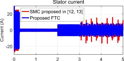


References Adaptive RBFNN strategy for fault tolerant control: application to DSIM under broken rotor bars fault
- N. Layadi, S. Zeghlache, T. Benslimane and F. Berrabah, “Comparative Analysis between the Rotor Flux Oriented Control and Backstepping Control of a Double Star Induction Machine (DSIM) under Open-Phase Fault,” AMSE Journals, Series Advances C, vol. 72, N 4, pp. 292–311, 2018.
- H. Rahali, S. Zeghlache and L. Benalia, “Adaptive field-oriented control using supervisory type-2 fuzzy control for dual star induction machine,” International Journal of Intelligent Engineering and Systems, vol. 10, N° 4, pp. 28-40, 2017.
- Z. Tir, Y. Soufi, M. N. Hashemnia, O. P. Malik and K. Marouani, “Fuzzy logic field oriented control of double star induction motor drive,” Electrical Engineering, vol. 99, N 2, pp. 495-503, 2017.
- M. Abd-El-Malek, A. K. Abdelsalam and O. E. Hassan,“ Induction motor broken rotor bar fault location detection through envelope analysis of start-up current using Hilbert transform,” Mechanical Systems and Signal Processing, vol. 93, pp. 332-350, 2017.
- R. A. Lizarraga-Morales, C. Rodriguez-Donate, E. Cabal-Yepez, M. Lopez-Ramirez, L. M. Ledesma-Carrillo and E. R. Ferrucho-Alvarez, “Novel FPGA-based Methodology for Early Broken Rotor Bar Detection and Classification Through Homogeneity Estimation,” IEEE Transactions on Instrumentation and Measurement, vol. 66, N 7, pp. 1760-1769.
- E. Elbouchikhi, V. Choqueuse, F. Auger and M. E. H. Benbouzid, “Motor Current Signal Analysis Based on a Matched Subspace Detector,” IEEE Transactions on Instrumentation and Measurement., vol. 66, N 12, pp. 3260-3270, 2017.
- Z. Hou, J. Huang, H. Liu, T. Wang and L. Zhao, ”Quantitative broken rotor bar fault detection for closed-loop controlled induction motors,” IET Electric Power Applications, vol. 10, N° 5, pp. 403-410, 2016.
- H. Yang and J. Liu, “An adaptive RBF neural network control method for a class of nonlinear systems,” IEEE/CAA Journal of Automatica Sinica, vol. 5, N 2, pp. 457-462, 2018.
- L. Zhu, Z. Wang, Y. Zhou and Y. Liu, “Adaptive Neural Network Saturated Control for MDF Continuous Hot Pressing Hydraulic System With Uncertainties,” IEEE Access, vol. 6, pp. 2266-2273, 2018.
- J. Zhi, Y. Chen, X. Dong, Z. Liu and C. Shi, “Robust adaptive FTC allocation for over-actuated systems with uncertainties and unknown actuator non-linearity,” IET Control Theory & Applications, vol. 12, N 2, pp. 273-281, 2017.
- S. Zeghlache, H. Mekki, A. Bouguerra and A. Djerioui, ”Actuator fault tolerant control using adaptive RBFNN fuzzy sliding mode controller for coaxial octorotor UAV,” ISA transactions, vol. 60, pp. 267-278, 2018.
- J. Listwan and K. Pieńkowski, ”Sliding-mode direct field-oriented control of six-phase induction motor,” Czasopismo Techniczne, vol. (2-M), pp. 95-108, 2016.
- M. A. Fnaiech, F. Betin, G. A. Capolino and F. Fnaiech, “Fuzzy logic and sliding-mode controls applied to six-phase induction machine with open phases,” IEEE Transactions on Industrial Electronics, vol. 57, N° 1, pp. 354-364, 2010.
- M. Manohar and S. Das, ”Current sensor fault-tolerant control for direct torque control of induction motor drive using flux-linkage observer,” IEEE Transactions on Industrial Informatics, vol. 13, N 6, pp. 2824-2833, 2017.
- H. Mekki, O. Benzineb, D. Boukhetala, M. Tadjine and M. Benbouzid, ”Sliding mode based fault detection, reconstruction and fault tolerant control scheme for motor systems,” ISA Transactions, vol. 57, pp. 340-351, 2015.
- S. Rubino, R. Bojoi, S. A. Odhano and P. Zanchetta, ”Model predictive direct flux vector control of multi three-phase induction motor drives,” IEEE Transactions on Industry Applications, vol. 54, N 5, pp. 4394 – 4404, 2018.
- N. Djeghali, M. Ghanes, S. Djennoune and J. P. Barbot, “Sensorless fault tolerant control for induction motors, ” International Journal of Control, Automation and Systems, vol. 11, N 3, pp. 563-576, 2013.
- N. Bounar, A. Boulkroune, F. Boudjema, M. M’Saad and M. Farza, “Adaptive fuzzy vector control for a doubly-fed induction motor,” Neurocomputing, vol. 151(Pt 2), pp. 756-769, 2015.
- I. González-Prieto, M. J. Duran and F. J. Barrero, “Fault-tolerant control of six-phase induction motor drives with variable current injection,” IEEE Transactions on Power Electronics, vol. 32, N 10, pp. 7894-7903, 2017.
- E. A. Mahmoud, A. S. Abdel-Khalik and H. F. Soliman, “An improved fault tolerant for a five-phase induction machine under open gate transistor faults,” Alexandria Engineering Journal, vol. 55, N 3, pp. 2609-2620, 2016.
- S. Bednarz, “Rotor Fault Compensation and Detection in a Sensorless Induction Motor Drive,” Power Electronics and Drives, vol. 2, N 1, pp. 71-80, 2017.
