Agent-Based Crowd Simulation of Daily Goods Traditional Markets

Author: Purba D. Kusuma, Azhari, Reza Pulungan
Journal: International Journal of Intelligent Systems and Applications(IJISA) @ijisa
Article in issue: 10 vol.8, 2016.
Free access
In traditional market, buyers are not only moving from one place to another, but also interacting with traders to purchase their products. When a buyer interacts with a trader, he blocks some space in the corridor. Besides, while buyers are walking, they may be attracted by non-preferred traders, though they may have preferred traders. These situations have not been covered in most existing crowd simulation models. Hence, these existing models cannot be directly implemented in traditional market environments since they mainly focus on crowd members' movement. This research emphasizes on a crowd model that includes simplified movement and unplanned purchasing models. This model has been developed based on intelligent agent concept, where each agent represents a buyer. Two traditional markets are used for simulation in this research, namely Gedongkuning and Ngasem, in Yogyakarta, Indonesia. The simulation shows that some places are visited more frequently than others. Overall, the simulation result matches the situation found in the real world.
Crowd, simulation, traditional market, intelligent agent
Short address: https://sciup.org/15010861
IDR: 15010861
Text of the scientific article Agent-Based Crowd Simulation of Daily Goods Traditional Markets
Published Online October 2016 in MECS
The number of traditional markets in Indonesia is declining. People change their shopping habit from traditional market to modern market. Traditional markets are perceived as a crowded environment; buyers cannot move easily; while the opposite happens in modern markets. In this case, crowd management is important for stakeholders to encourage people to shop at traditional markets. Simulation technology can be used to systematically study crowd management in traditional markets. By using simulation, stakeholders can observe and predict the situation in traditional markets even before they are built.
Unfortunately, a crowd simulation model for traditional markets cannot be straightforwardly developed based on existing crowd simulation models. Many existing models focus mainly on the movement of the crowd’s members. A crowd in traditional markets, on the other hand, is not only affected by buyers’ movement but also buyers’ interaction with traders.
The purpose of this research is to propose and develop a new crowd simulation model for traditional markets. Two steps are involved in developing this model. The first is to develop a model that captures buyers’ movement as well as their decision making process. The second step is to implement the resulting model into a crowd simulation. The environment of the crowd simulation is, however, limited to the daily goods traditional markets in Yogyakarta, Indonesia.
This paper is organized as follows. Section I describes the problem statement, the research purpose, and the organization of the paper. Section II provides the overview of the significant work in the field. Section III explains the proposed model. Section IV describes the simulation scenario. Section V presents resulting data produced by the simulation and then analyzes them. Section VI concludes the paper.
-
II. R ELATED W ORK
There are many methods that can be used to develop crowd models, such as: particle system, fluid, flock, or autonomous agent [1]. Flock concept is adopted based on animals’ movement in a certain group, such as birds or fishes [2]. In fluid concept, crowd is modeled as rigid tiles that move from one point to another [3]. This concept is similar to the particle system concept [4]. The main advantage of using those models is the simplicity of the calculation, which makes their computation easier [3]. The main problem, on the other hand, is that the models cannot represent human crowd realistically, because they lack ability to model intention and logical thinking, which are involved during human’s decision making process.
Human crowds can be modeled more realistically when they are based on agent concept. In agent-based approach, crowd members must think and make decision before moving [5-7]. Moreover, agent based approach allows psychological aspect to be included in the reasoning process.
One popular movement model is the social forces model [8]. This model is closer to human walking behavior compared to those of fluid mechanics or particle system [9]. Four forces are implemented in this model: desired movement force, interaction force, wall avoidance, and attracting force. One popular system that uses this model is HiDAC [6]. HiDAC has been used as simulation tool for many researches [5, 10, 11].
Beside social forces model, cellular automata are also popular in crowd simulation modeling. This method is widely used because it is simple and light. Different from social forces model, cellular automata use a discrete approach [12]. Some crowd simulations that use cellular automata are focused on panic situations and evacuations [12,13]. Some cellular automata-based crowd models also use a multi-agent approach [12-15].
-
III. P ROPOSED M ODEL
In the proposed crowd simulation, cellular automatabased pedestrian dynamics is implemented and combined with social forces concept. Different from social forces model, however, buyers usually walk in constant speed because they walk in narrow corridors. Nevertheless, buyers’ speed may be different from each other. Stop and go concept can then be applied: when space is enough, they walk; when space is not enough, they stop. There are booths on the left and right sides of each corridor. So, there are repulsive forces from their left and right sides . Since the forces are equal, buyers tend to walk in the middle of the corridor. When a buyer meets another buyer, they tend to move to the empty space nearest to them to avoid collision. The empty space can be to the buyer’s left, right, front-left, or front-right sides.
In our proposed simulation, intelligent agents model the buyers. A buyer’s existence in the environment is dynamic: its existence starts when the buyer enters the market and ends when she leaves the market. The buyer’s position is dynamic too, because during a visit to the market, a buyer moves from one booth to another, until her mission is accomplished. While buyer is in the market, she visits traders. A trader’s existence in the environment is, however, static: it exists from when the simulation begins until it ends. During the simulation, the trader’s spatial position is static too, namely her position is in her booth.
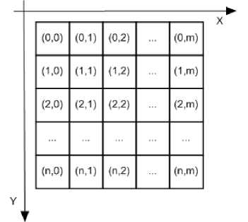
Fig.1. Illustration of the grid model
A traditional market environment is therefore represented by a two dimensional grid. The grid coordinate system’s axes are x for horizontal and y for vertical directions. The top-left position corresponds to coordinate (0,0). A single cell represents a 20 cm x 20 cm tile in the reality. The grid model is depicted in Fig. 1. The maximum values of x and y are m and n , respectively.
Each agent representing a buyer occupies a single cell. An agent I is represented by variable B with index i ( B i ). The time step is represented by variable t . We use p(Bi,t) to denote the coordinate of the position of agent i at time t . The agent’s movement is determined by the target position p(Ti,t) and the agent’s neighbors. Let A be the set containing agent B i ’s neighbor cells. There are 8 members in set A denoted by a 1 , a2, ..., a8 . Let p(a j ) be the coordinate of the position of neighbor cell j . Furthermore, let s(a j ) denote the state of neighbor cell j , namely it is 0 when the cell is free and 1 when the cell is occupied.
An agent can move only to one of its neighbor cells that is free. If there is no free neighbor cell, the agent will stay at its position at the time t . The agent together with its eight neighbors are depicted in Fig. 2. The movement procedure is deterministic and it is described by Equations (1)-(3). Equation (1) describes the distance between the agent’s target position to each of its neighbor cells. Equation (2) specifies a set fl containing all free neighbor cell. Equation (3) describes the coordinate of the next position of agent Bi at time t+1 .
dj (t)= b(a > )-P(7 i ,t)y (1)
fl = {aJs(a ; ) = 0} (2)
( p(a^, min7-{ d ((t}^ and. s( a )) e fl
" Ip(S^t), fl = 0
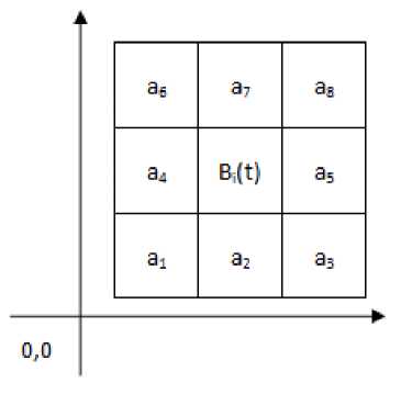
Fig.2. The agent and its eight neighbors
The next step is the agent’s decision making model related to attracting objects near itself. The attracting object does not have any direct effect to the next tile to which the agent will move. However, it may change the agent’s target. In this model, the attracting objects are the booths near a buyer, where products that the buyer plans to buy are being sold. For example, the buyer may plan to purchase a chicken from trader A. Trader A is the buyer’s preferred trader for chicken. Then, while the buyer is walking to trader A, she may see that there are other traders selling chicken too. The agent representing the buyer may then change its target.
There are 2 parameters that affect the agent’s decision making process related to the attracting object. The first is the buyer’s loyalty to her preferred trader. This loyalty value may be different between buyers or traders. It can be said that when this loyalty factor is high, the buyer’s resistance from her non-preferred trader’s proposal is high too. The second is a trader’s attractiveness. When the trader is more attractive, the probability that the buyer changes her target is higher.
The buyer changes her target to a non-preferred trader if the trader’s position is in the buyer’s observation range and the trader’s attractiveness value is higher than the buyer’s loyalty factor, and the trader sells the same product group as the buyer’s preferred trader. If there are more than one trader complying with these conditions, then the buyer will move to the trader with highest attractiveness value.
The movement procedure is deterministic and explained in Equations (4)-(7). Let r denote the radius of the buyer’s observation range ( cf. Fig. 3). Let p(m j ) be the coordinate of the position of trader m j . The distance between buyer B i ’s position at time t and trader m j ’s position is given by Equation (4). Let T(t) denote buyer B i ’s target at time t , and gr(m j ) denote the product group of trader m j . Equation (5) describes M , the set of all traders in buyer B i ’s observation range, whose product group matches buyer B i ’s target product group. Let at(m j ) denote trader m j ’s attractiveness value, and ly(B i ) denote buyer B i ’s loyalty factor. Equation (6) describes g j , the difference between m j ’s attractiveness value and B i ’s loyalty factor. Equation (7) describes B i ’s target at time t+1 .
This can be trader’s position or the location of an exit. It is denoted by l . The second is a primary checkpoint denoted by p , a member of set P . The third is a secondary checkpoint denoted by s , a member of set S . The fourth is an escape exit checkpoint denoted by e , a member of set E . The position of the primary, secondary, and escape checkpoints is illustrated in Fig. 5. The position of the primary checkpoint is in the center of the crossing point ( cf. Fig. 5(a)). The position of the secondary checkpoints is in the center of the booth corridors ( cf. Fig. 5(b)). The position of the escape checkpoints is in front of each trader’s booth ( cf. Fig. 5(c)).
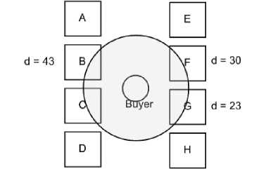
Fig.3. Buyer’s observation range begin m ←settarget(B);
T ← setcheckpoint(m);
while(p(B) * p(m))
if (p(B) * p(T))
walk(B, m);
else
T ← setcheckpoint(m);
if (cannotwalk(B) = true) T ← setcheckpoint(m);
end
Fig.4. The algorithm of the routing process dj (t)= b(my)-p(Bi,t)y
M = {my|gr(mj) = gr(T(t)) and d((t)< r](5)
Si = at(m.j') - ly(B)(6)
T (t + 1) = {
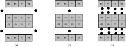
Fig.5. Checkpoint position
THj, max , Ь } and g, > 0
T Ct), M = 0 о r ^j. g j < 0
Routing is used to determine the path used by the agent to reach its target. Routing mechanism used in this research is based on the checkpoint model. The routing mechanism does not store a path used by the agent. Therefore, the next cell that will be occupied at time t+1 is always calculated at time t . This method is chosen to reduce memory consumption. The agent always observes its actual and current environment. The algorithm of the routing process is depicted in Fig.4.
There are 4 checkpoint types. The first is the real target.
T(t) = {с | с e P and min j {^p(c) - p(m j )||}} (8)
T(t) = {c | e E a nnd min^lpCc) - p(m y )|}} (9)
T(t) = {rand(c) I c e E and Hp(c) - p(Bt, t)H < r}
The routing process runs sequentially. The first step is the target determination, which is the next trader’s position or the exit location. After the target is determined, then the agent will determine its primary checkpoint. The primary checkpoint chosen is the closest primary checkpoint to the target. For a checkpoint c, let p(c) denote the coordinate of its position. The primary checkpoint determination is given by Equation (8). After the primary checkpoint is determined then agent will head in that direction. After the agent reaches its primary checkpoint, the agent will determine his secondary checkpoint. The secondary checkpoint chosen is the closest secondary checkpoint to the target. The secondary checkpoint determination is given by Equation (9). After the secondary checkpoint is determined, then the agent will head in that direction. After the agent reaches his secondary checkpoint, the agent will then proceed to its real target. While the agent is walking, if it encounters an unmovable obstacle, it will determine its escape checkpoint. Escape checkpoint determination is given by Equation (10). The variable r in Equation (10) represents the radius of the agent’s observation range. The random method follows uniform distribution. After the agent reaches its escape checkpoint, the agent will proceed to its previous target, even though it is a primary checkpoint, a secondary checkpoint, or the real target. After the agent reaches its real target, the walking and routing processes stop.
-
IV. S IMULATION
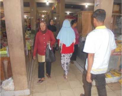
Traditional markets used in this simulation are Gedongkuning and Ngasem market. They are daily goods markets, located in Yogyakarta, Indonesia. A daily goods market is a market that sells daily products, such as food, vegetables, snack, and kitchen tools. Fig. 6 shows pictures of the two markets.
Several characteristics are prevalent in daily goods traditional markets. First, traders sell similar type of products, as they are catering for daily consumption. Therefore, the difference in price for the same products among traders is not significant. The pricing mechanism in this situation is a combination between cost-based price and competition-driven price [16]. Hence, the price negotiation between buyers and traders is not hard. In many cases, buyers do not negotiate the price. Second, each buyer usually has a preferred daily goods traditional market and visits frequently. This allows the buyer to remember the site plan of her preferred market. Third, each buyer usually has a preferred trader for every product. So, the buyer will first go to her preferred traders rather than to other traders that provide the same product. This behavior is similar to brand consciousness in customer behavior model. If a product is a commodity, the brand means the trader [17]. However, even though a buyer has preferred traders, this is not a blind commitment. Sometimes the buyer may choose a nonpreferred trader [18], for instance, because the nonpreferred trader’s display quality [19] or the preferred trader cannot provide the product that the buyer needs.
There are 2 corridor types in a typical traditional markets: main corridors and booth corridors. Fig. 3 shows the illustration of a booth corridor. Main corridors are the corridors near to the entrance or the exit gates. They are used by buyers to move from one area to another in the market. Booth corridors are the corridor between booths. When buyers interact with traders, they usually stand on a booth corridor. Main corridors are wider than booth corridors. Based on visual observation, crowds usually occur in booth corridors rather than in main corridors.
In Gedongkuning market, the main corridors are longer than booth corridors, while in Ngasem market, main corridors are shorter than booth corridors. In Ngasem, the main corridors are usually empty because buyers walk more often in booth corridors. This condition is different from that in Gedongkuning. In Gedongkuning, buyers almost always use the main corridors to move from one booth to others.
There are several empty booths in Gedongkuning or Ngasem market. More empty booths are found in Ngasem than in Gedongkuning. In Ngasem market, two blocks have a lot of empty booths. The crowd density in the corridors around the empty booths is lower than those around non-empty booths.
(a)

(b)
Fig.6. (a) Gedongkuning and (b) Ngasem markets
The condition near the entrance and exit gates is also different in Gedongkuningfrom that in Ngasem. In Gedongkuning, crowd density in corridors near the gates is higher than those far from the gates. In Ngasem, crowd is found more often in the center corridors rather than in the corridors near or far from the gates.
There are 80 booths in Gedongkuning. The distribution of the booths based on the product groups is shown in Table 1. Several parameters are selected to be used in the simulation, and these are based on field survey in Gedongkuning. The buyer arrival rate is set to 5.3 buyers per minute. The buyer’s walking speed ranges from 0.54 to 1.4 meters per second. The buyer-trader engagement duration ranged from 35 to 239 seconds. The number of buyer’s visitation ranged from 1 to 5 traders.
In Ngasem, there are 108 booths. The distribution of the booths based on the product groups can be seen in Table 2. Based on field survey in the lower ground in Ngasem, there exist 3 entrance gates. The arrival rate at the first, second, and third gates is 3.4, 2.2, and 1.8 buyers per minute, respectively. In the simulation, other parameters, such as the arrival interval and buyer-trader engagement duration are the same as those of Gedongkuning.
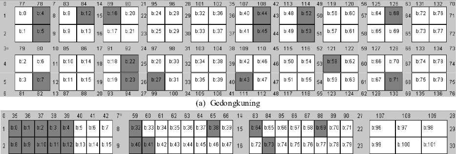
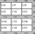
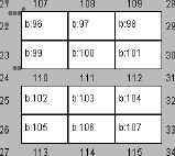
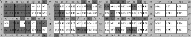
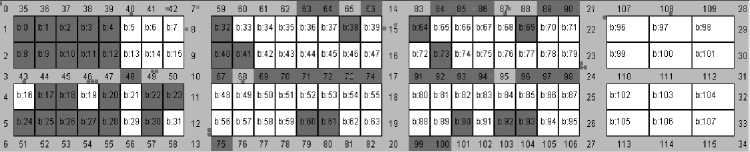
The site plan of Gedongkuning and Ngasem markets is depicted in Fig. 7. The explanation of the site maps is as follows. The light gray area represents corridors. The white blocks represent non-empty booths. The gray blocks represent empty booths. The number in the corridor represents the corridor number. The number in the booth represents the booth number.
3 43 44 45 46 47 48 49 50 1 0 67 68 69 70 71 72 73 74 1 7 91 92 93 94 95 96 97 98 24 1 10 1 1 1 1 12 31
|
b:16 |
b:17 |
b:18 |
b:19 |
b:20 |
b:21 |
b:22 |
b:23 |
|
b:24 |
b:25 |
b:26 |
b:27 |
b:28 |
b:29 |
b:30 |
b:31 |
|
b:48 |
b:49 |
b:50 |
b:51 |
b:52 |
b:53 |
b:54 |
b:55 |
|
b:56 |
b:57 |
b:58 |
b:59 |
b:60 |
b:61 |
b:62 |
b:63 |
|
b:80 |
b:81 |
b:82 |
b:83 |
b:84 |
b:85 |
b:86 |
b:87 |
|
b:88 |
b:89 |
b:90 |
b:91 |
b:92 |
b:93 |
b:94 |
b:95 |
|
b:102 |
b:103 |
b:104 |
|
b:105 |
b:106 |
b:107 |
6 51 52 53 54 55 56 57 58 1 3 75 76 77 78 79 SO 81 82 20 99 1 00 101 1 02 1 03 1 04 105 106 27 1 13 1 1 4 1 15 34
-
(b) Ngasem
-
Fig.7. Market site plan
Table 1. Traders distribution in Gedongkuning
|
Product Group |
Booth Number |
|
Burner |
3. |
|
Vegetables |
2, 6, 21, 29, 36, 40, 48, 59. |
|
Fruits |
1, 19, 31. |
|
Seasoning |
8, 9, 11, 20, 28, 30, 32, 33, 34, 35, 37, 38, 42, 46, 50, 54, 55. |
|
Tempe |
10, 15, 17, 26, 57. |
|
Kitchen tools |
13, 14, 51. |
|
Snacks |
0, 18, 25, 39, 41, 47, 49. |
|
Chicken |
56, 60, 61, 62, 64, 65, 66, 69, 70. |
|
Beef |
63. |
|
Fish |
67, 72, 73, 74, 75, 76, 77, 78, 79. |
|
Rice |
24. |
|
Empty booths |
4, 5, 7, 12, 16, 22, 23, 27, 43, 44, 45, 52, 53, 58, 68, 71. |
Experiments are conducted by running the simulation for an hour in real situation for each cycle. The number of customers that enter the market in every arrival cycle is varied. Based on that varied number, the simulations can be divided into 3 groups: the first group corresponds to one customer in each cycle, the second corresponds to one to two customers in each cycle, and the third corresponds to one to three customers in each cycle. For each group, five simulation cycles are performed.
Four procedures are run when a simulation cycle is started. The procedures are for setting up simulation parameters, market site map, traders’ parameters, and customers’ parameters. The simulation parameters consist of simulation duration and arrival interval.
A buyer’s activity when she is in the market is described as follows. First, the buyer enters the market from the entrance/exit gate. In the market, the buyer visits her preferred traders based on her buying list. When buyer has completed her buying list, she leaves the market by walking to the exit gate. If there are more than one gate in the market, the buyer chooses the gate closest to her. There is a possibility that a buyer leaves the market before completing her list. While the buyer is walking in the market, she might be attracted by her nonpreferred traders. When the buyer’s time in the market has reached the maximum staying time, the buyer decides to leave the market before completing her buying list.
Table 2. Traders distribution in Ngasem
|
Product group |
Booth number |
|
Fruits |
21, 29, 37, 56, 67, 71, 81, 89. |
|
Vegetables |
6, 7, 13, 14, 15, 33, 34, 35, 36, 39, 44, 45, 47, 50, 52, 55, 57, 58, 68, 72, 74, 76, 77, 78, 79, 80, 82, 84, 86, 87, 95. |
|
Tempe |
5, 31, 46, 51, 70, 75, 83, 94. |
|
Seasoning |
42, 43, 48, 49, 53, 54, 59, 62, 63, 85, 96, 97, 98, 99, 100, 101, 102, 103, 104, 105, 106, 107. |
|
Kitchen tools |
16, 19, 88, 91. |
|
Eggs |
65, 66. |
|
Empty booths |
0, 1, 2, 3, 4, 8, 9, 10, 11, 12, 17, 18, 20, 22, 23, 24, 25, 26, 27, 28, 30, 32, 38, 40, 41, 60, 61, 64, 69, 73, 90, 92, 93. |
V. R ESULT AND D ISCUSSION
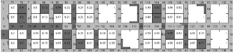
The first result concerns the corridors, in which crowds are observed during the simulation. The aim of this simulation is to find the consistency of the crowd that occurs in the corridors across simulation cycles, even when the trader’s attractiveness level was varied in every simulation cycle. The resulting data is analyzed to find the correlation between crowd probability and the location of the corridors. The result is presented in Table 3 for Gedongkuning and Table 4 for Ngasem. There are 4 columns in these tables. The first column is the number of simulation cycles, where crowds are observed. The second, third and fourth columns each lists corridors for the first, second, and groups, respectively. A visual representation of the crowd occurrences during the simulation can be seen in Fig. 8 for Gedongkuning and Fig. 9 for Ngasem.
Table 3 indicates that all crowds occur in booth corridors. When the probability of the people entering the market is higher, the probability that crowds occur in main corridor is also higher. This can be observed in the third column (second group) and in the fourth column (third group). In the second group, the main corridors of the observed crowds are in corridors 10, 91, 97, 98, 103, 109, 115, 116, and 122. The ratio between the number of the main corridors and all corridors where the crowds are observed is 47 percent for the second group. In the third group, the main corridors where crowds are observed are corridors 45, 92, 97, 98, 52, 59, 85, 86, 91, 122, 38, 31, 10, 17, 24, and 79. The ratio between the number of main corridors and all corridors where crowds are observed is 53 percent for the third group. Therefore, in Gedongkuning crowds occur more frequently in booth corridors than in main corridors.
Based on the distance to the entrance-exit gate, the probability of a crowd to occur in a corridor is higher when it is closer to the gate. The gate is located in corridor 3. Based on the distance from the corridor to the gate, the corridors can be divided into 2 groups : the first group is the corridors around booths 0 to 39, while the second group is the corridors around booths 40 to 79. Corridors 35 to 41 are excluded because they are right in the middle. The second column in Table 3 indicates that 6 corridors are in the first group and 1 corridor is in the second group. The ratio is therefore 6. The third column in Table 3 indicates that 11 corridors are in the first group and 6 corridors are in the second group. The ratio is 1.8. The fourth column in Table 3 shows that 22 corridors are in the first group and 6 corridors are in the second group. The ratio is 3.7. Based on these ratios, we conclude that the population size does not affect the crowd distribution.
Table 3. Corridors in Gedongkuning where crowds are observed
|
Number of Cycles |
Corridors |
||
|
1 st group |
2 nd group |
3 rd group |
|
|
1 |
19, 33, 61. |
37, 38, 45, 59, 79, 91, 97, 98, 103, 109, 115, 116, 122. |
37, 45, 80, 92, 97, 98. |
|
2 |
9, 18. |
9, 10, 32 |
39, 52, 59, 85, 86, 91, 122. |
|
3 |
22, 23. |
23. |
9, 16, 30, 38. |
|
4 |
18, 22. |
11, 31, 32, 33, 60. |
|
|
5 |
10, 17, 18, 19, 22, 23, 24, 61, 79. |
||
Table 4. Corridors in Ngasem where crowds are observed
|
Number of Cycles |
Corridor number |
||
|
1 st group |
2 nd group |
3 rd group |
|
|
1 |
66, 69, 71, 72, 74, 86, 92, 93. |
|
16, 17, 61, 62, 68, 75, 102. |
|
2 |
64, 70, 99. |
48, 66, 68, 69, 71, 72, 74, 96, 100. |
42, 58, 63, 90. |
|
3 |
67, 85, 94, 96. |
64, 93, 98, 99. |
46, 48, 66, 87, 100. |
|
4 |
73. |
70, 86, 92, 97. |
60, 64, 69, 91, 95, 96, 98. |
|
5 |
84. |
67, 73, 84, 85, 94. |
|
(a)
|
и |
I'Ll |
7 |
83 |
84 |
14 |
Ijg |
90 |
21 |
95 |
8b |
21 |
181 |
102 |
35 |
1 Of |
188 |
42 |
113 |
114 |
41 |
11 9 |
128 |
5 |
125 |
12b |
03 |
1 31 |
1 32 |
70 |
|
|
1 |
b:0 |
b:4 |
В |
b:8 |
b:12 |
15 |
b:16 |
b:28 |
29 |
b:32 |
b:36 |
30 |
b:40 |
b:44 |
43 |
b:48 |
b:52 |
50 |
b:56 |
b:60 |
5 |
b:64 |
b:68 |
04 |
b:72 |
b:76 |
71 |
|||
|
2 |
b:1 |
b:5 |
£ |
b:9 |
b:13 |
16 |
b:17 |
b:21 |
23 |
b:29 |
30 |
b:33 |
b:37 |
31 |
b:41 |
b:45 |
44 |
b:49 |
b:53 |
51 |
b:57 |
b:61 |
5 |
b:65 |
b:69 |
05 |
b:73 |
b:77 |
72 |
|
|
3- |
79 |
■80 |
10 |
85 |
86 |
17 |
91 |
92 г |
24 |
97 |
98 |
31 |
103 |
104 |
38 |
109 |
110 |
45 |
115- |
1W |
52 |
121 |
122 |
5 |
127 |
128 |
64 |
*33 |
134 |
73 |
|
4 |
b:2 |
b:6 |
b:14 |
b:18 |
b:22 |
25 |
b:26 |
b:30 |
32 |
b:34 |
b:38 |
39 |
b:42 |
b:4 6 |
40 |
b:54 |
53 |
b:62 |
6 |
b:70 |
07 |
b:74 |
b:78 |
74 |
||||||
|
5 |
b:3 |
12 |
b:11 |
b:15 |
- |
b:19 |
b:23 |
20 |
b:27 |
b:31 |
33 |
b:35 |
b:39 |
40 |
b:43 |
b:47 |
47 |
b:51 |
b:55 |
5» |
b:63 |
6 |
b:67 |
b:71 |
03 |
b:75 |
b:79 |
75 |
||
|
h |
8j |
87 |
88 |
93 |
94 |
27 |
99 |
1 00 |
32 |
105 |
1 06 |
41 |
111 |
112 |
4£ |
117 |
118 |
55 |
123 |
124 |
h |
1 29 |
130 |
69 |
1 35 |
1 36 |
76 |
(c)
|
0 |
77 |
78 |
7 |
83 |
84 |
14 |
89 |
90 |
21 |
95 |
96 |
21 |
101 |
102 |
35 |
107 |
108 |
42 |
113 |
114 |
49 |
119 |
120 |
5E |
125 |
126 |
6; |
131 |
132 |
70 |
|
M |
b:4 |
0 |
b:8 |
b:12 |
15 |
b:16 |
b:20 |
22 |
b:24 |
b:28 |
20 |
b:32 |
b:36 |
36 |
b:40 |
b:44 |
43 |
b:48 |
b:52 |
50 |
b:56 |
b:60 |
57 |
b:64 |
b:68 |
64 |
b:72 |
b:76 |
71 |
|
|
b:1 |
b:5 |
9 |
b:9 |
b:13 |
1» |
b:17 |
b:21 |
23 |
b:25 |
31 |
b:33 |
b:37 |
37 |
b:41 |
b:45 |
44 |
b:49 |
b:53 |
51 |
b:57 |
b:61 |
58 |
b:65 |
b:69 |
6| |
b:77 |
72 |
|||
|
3* |
79 |
80 |
10 |
85 |
86 |
17 |
91 |
92 |
24 |
97" |
ЗД- |
81 |
103 |
*34 |
38 |
109 |
110 |
45 |
115* |
1K |
52 |
*21 |
122 |
59 |
127 |
128 |
66 |
133 |
134 |
73 |
|
4 |
b:2 |
b:6 |
b:10 |
b:14 |
b:22 |
25 |
32 |
b:38 |
33 |
b:42 |
b:46 |
46 |
b:50 |
b:54 |
53 |
b:58 |
b:62 |
til |
b:66 |
b:70 |
67 |
b:74 |
b:78 |
74 |
||||||
|
5 |
b:3 |
b:7 |
12 |
b:11 |
b:15 |
b:23 |
20 |
■ |
33 |
b:35 |
b:39 |
40 |
b:43 |
b:47 |
47 |
b:51 |
b:55 |
54 |
b:59 |
b:63 |
■61 |
b:67 |
b:71 |
60 |
b:75 |
b:79 |
75 |
|||
|
0 |
81 |
R9 |
87 |
RR |
94 |
27 |
1 RR |
Rd |
105 |
1 OR |
4 ■ |
111 |
11 ‘j |
4f |
117 |
11 R |
55 |
1 98 |
1 74 |
R7 |
179 |
1 90 |
RC |
145 |
1 RR |
7R |
(d)
|
b:32 |
b:36 |
|
b:33 |
b:37 |
|
b:40 |
b:44 |
|
b:45 |
|
b:46 |
|
|
b:43 |
b:47 |
|
b:64 |
b:68 |
|
b:69 |
|
b:72 |
b:76 |
|
b:73 |
b:77 |
|
b:74 |
b:78 |
|
b:79 |
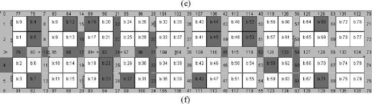
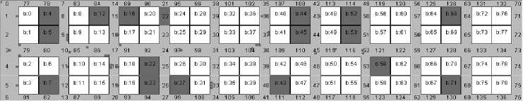
Fig.8. Visual presentation of the simulation result in Gedongkuning
There is also a correlation between the probability of crowd occurrences and the product group being sold in the booths between the corridors. The corridors can be divided into 3 groups: the first group consists of corridors located between booths with different product group, the second group consists of corridors located between booths with the same product group, and the third group consists of corridors located beside empty booths. The first column in Table 3 shows that 6 corridors are in the first group and 1 corridor is in the third group. We can conclude that probability of crowd occurrences in corridors in the first group is higher than that in the second or third group.
(a)
|
b:0 |
b:1 |
b:2 |
b:3 |
b:4 |
b:5 |
b:6 |
b:7 |
|
b:8 |
b:9 |
bio |
b:11 |
b:12 |
b:13 |
b:14 |
b:15 |
|
b:16 |
b:17 |
b:18 |
b:19 |
b:20 |
b:21 |
b:22 |
b:23 |
|
b:24 |
b:25 |
b:26 |
b:27 |
b:28 |
b:29 |
b:3O |
b:31 |
|
b:32 |
b:33 |
b:34 |
b:35 |
b:36 |
b:37 |
b:38 |
b:39 |
|
b:40 |
b:41 |
b:43 |
b:44 |
b:45 |
b:46 |
b:47 |
|
|
67 |
68 69 |
70 |
71 72 7^ 74 |
||||
|
b:48 |
b:49 |
b:50 |
b:51 |
b:52 |
b:53 |
b:54 |
b:55 |
|
b:56 |
b:57 |
b:58 |
b:59 |
b:60 |
b:61 |
b:62 |
b:63 |
(b)
|
b:64 |
b:65 |
b:66 |
b:67 |
b:68 |
b:69 |
b70 |
b71 |
|
Ь72 |
b:73 |
1)74 |
Ь75 |
b:76 |
b77 |
Ь78 |
Ь79 |
|
b:8O |
b:81 |
b:82 |
b:83 |
b:84 |
b:85 |
b:86 |
b:87 |
|
b:88 |
b:89 |
b:90 |
b:91 |
b:92 |
b:93 |
b:94 |
b:95 |
(c)
|
b:0 |
b:1 |
b:2 |
b:3 |
b:4 |
b:5 |
b:6 |
b:7 |
|
b:8 |
b:9 |
b:10 |
b:11 |
b:12 |
b:13 |
b:14 |
b:15 |
|
b:16 |
b:17 |
b:18 |
b:19 |
b:20 |
b:21 |
b:22 |
b:23 |
|
b:24 |
b:25 |
b:26 |
b:27 |
b:28 |
b:29 |
b:30 |
b:31 |
|
b:32 |
ь:зз |
b:34 |
b:35 |
b:36 |
b:37 |
b:38 |
b:39 |
|
b:4O |
u:41 |
b:43 |
b:44 |
b:45 |
b:46 |
b:47 |
|
|
67 68 69 70 |
71 72 |
73 |
74 |
||||
|
b:48 |
b:49 |
b:50 |
b:51 |
b:52 |
b:53 |
b:54 |
b:55 |
|
b:56 |
b:57 |
b:58 |
b:59 |
b:60 |
b:61 |
b:62 |
b:63 |
(d)
(e)
(f)
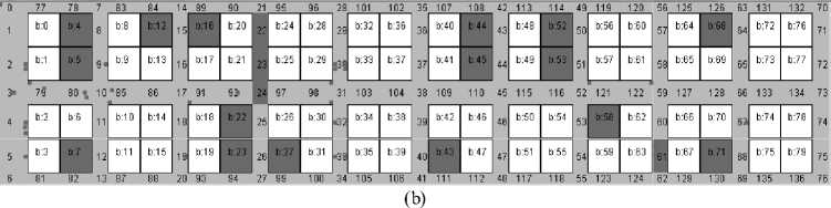
Fig.9. Visual presentation of the simulation result in Ngasem
Crowd visualization in Gedongkuning is presented in Fig. 8. These figures are captured during simulation where arrival interval is set to 12 seconds. Fig. 8(a) and (b) represent crowds for the first group; Fig. 8(c) and (d) represent crowds for the second group, and Fig. 8(e) and (f) represent crowds for the third group. These figures strengthen the analysis that crowds occur more often near the gate rather than far from gate. They also strengthen the analysis that for low traffic, crowds occur more often in booth corridors. But when the traffic is higher, crowds occur in the main corridors too.
In the first group in Table 4, all crowds are observed in the booth corridors. There is no crowd observed in the main corridors (corridors 0 to 34). This condition occurs for the first, second, and third groups. Based on the explanation above, both in Gedongkuning and Ngasem, there is a correlation between the probability of crowd occurrences and and the type of the corridor. Crowds occur more frequently in booth corridors than in main corridors. Buyers will use the main corridor when they enter and leave the market, and use it many times to move from one booth to another booth; hence, crowds never occur in the main corridor. One possible explanation is the corridor width and human behavior in this corridor. The main corridor is wider than booth corridors, people can move easier there than in booth corridors. In the main corridor, more buyers walk rather than stand still, while in booth corridors, more buyers stand still and interact with the traders. This condition makes the probability of crowd occurrences in booth corridor is higher than in the main corridor. This simulation result matches the situation found in the real world.
The next analysis is about the distribution of the crowds based on the distance to the entrance-exit gates. There are three groups: near, middle, and far. In the first group in Table 4, 29 percent is near, 64 percent is middle, and 5 percent is far. In the second group in Table 4, 34 percent is near, 53 percent is middle, and 12 percent is far. In the third group in Table 4, 39 percent is near, 47 percent is middle, and 13 percent is far.
From the explanation above, in Ngasem, crowds most frequently occur in the middle group. The reason is there are two booths beside each corridor. In the near and far groups, there is only one booth beside each corridor. Hence, the probability that buyers are in the middle group is highest among all corridor groups based on the distance to the entrance-exit gates. The near group is the second highest because those corridors are near the gate and buyers enter or leave the market through the gate.
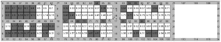
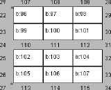
The crowd visualization strengthens the analysis above. This can be observed in Fig. 9. Fig. 9(a) and (b) are visualization for the first group, Fig. 9(c) and (d) are visualization for the second group, and Fig. 9(e) and (f) are visualization for the third group. It can be seen that in Ngasem, crowds occur in booth corridors, not in main corridors. Crowd occurs most often in the middle horizontal corridors, then in the top corridors, and in the bottom corridors.
Based on the product group in the booths between the corridors, corridors can be divided into 3 types. The first type is corridors with the booths selling different product group; the second type is corridors with the booths selling the same product group; and the third group is corridors with empty booths. Table 5 indicates that in all groups, crowds occur least frequently in the third type corridors. In the first group, crowds occur most frequently in the first type corridor. In the second and third groups, crowds occur most frequently in the second type corridor. We can conclude that in Ngasem, the probability of crowd occurrences is high in the corridors with no empty booths beside nearby.
The last data is about the crowd duration. The crowd duration is calculated by summing all crowd duration in all corridors in every simulation cycle. The crowd duration is presented in minutes. The purpose is to find the number of buyers entering the market in every arrival cycle. The result can be seen in Table 5 and 6.
Table 5. Crowd duration in Gedongkuning
|
Cycle number |
Crowd duration (minutes) |
||
|
1 st group |
2 nd group |
3 rd group |
|
|
1 |
2.74 |
29.57 |
53.73 |
|
2 |
0.01 |
13.09 |
37.20 |
|
3 |
2.01 |
10.67 |
32.19 |
|
4 |
11.53 |
8.29 |
51.28 |
|
5 |
10.22 |
11.85 |
36.07 |
Table 6. Crowd duration in Ngasem
|
Cycle number |
Crowd duration (minutes) |
||
|
1 st group |
2 nd group |
3 rd group |
|
|
1 |
1.64 |
13.44 |
38.81 |
|
2 |
1.89 |
21.93 |
45.75 |
|
3 |
0.98 |
18.21 |
41.55 |
|
4 |
2.88 |
14.09 |
51.63 |
|
5 |
5.29 |
17.48 |
43.55 |
Based on the field observation, crowd duration in Ngasem ranges approximately from 20 to 30 minutes in one hour. Crowd duration in the first group is far from the reality. Crowd duration in the second group is closer to the reality. The second cycle is in the range and the others are below the range. The second group are far above the range. Therefore, in Ngasem, the number between 1 and 2 for the number of buyers entering the market is close to the reality. On the other hand, crowd duration in Gedongkuning market is approximately 5 minutes in one hour. It can be seen that crowd duration in the first group in Table 6 is close to the reality. Therefore, in Gedongkuning, one buyer per arrival internal entering the market is close to the reality.
-
VI. C ONCLUSION
Based on the previous sections, we conclude that the proposed model has been implemented in crowd simulation for daily goods traditional markets. Crowds occur more frequently in booth corridors rather than in the main corridor. In Gedongkuning, crowds occur most often in corridors with booths selling varying product groups. In Ngasem, crowds occur more often in the corridors with no empty booths. In Gedongkuning, crowds occur more frequently in the corridors near to the entrance gate rather than far from the entrance gate. On the other hand, in Ngasem, crowds occur most frequently in the middle corridors rather than in the top or bottom corridors. Based on the simulation, the situation produced by the simulation is close to the real situation in the traditional markets. In Gedongkuning, one buyer per arrival interval is close to the reality. On the other hand, in Ngasem, one to two buyers per arrival interval is close to the reality.
Some improvements can be carried out to make the simulation more realistic : implementation of unplanned purchasing, implementation of negotiation process between buyers and traders and measuring the impact of the negotiation to the engagement duration, and the improvement in path planning to fix the problem that is explained in this paper. One of the conclusions of this paper is that the arrival rate does not give linear effect to the crowd condition. Some parameters such as engagement duration between buyers and traders, customer loyalty, and trader attractiveness have not been explored. It will be challenging to explore these parameters and evaluate them with the correlation to the crowd condition.
References Agent-Based Crowd Simulation of Daily Goods Traditional Markets
- R. Parent, “Computer Animation: Algorithms and Techniques”, San Francisco, Morgan Kaufmann Publishers, 2002.
- O.B. Bayazit, J.M. Lien, and N.M. Amato, “Better Group Behaviors in Complex Environments Using Global Roadmaps”, Proceeding of Artificial Life, Massachusetts, 2002, pp.1-10.
- S. Chenney, “Flow Tiles”, SIGGRAPH, 2004, pp.232-242.
- E. Bouvier, E. Cohen, and L. Najman, “From Crowd Simulation to Airbag Deployment: Particle Systems, a New Paradigm of Simulation”, Journal of Electronic Imaging, vol. 6, 1997, pp.94-107.
- F. Durunipar, “From Audiences to Mobs: Crowd Simulation with Psychological Factors”, Department of Computer Engineering, Bilkent University, 2010, Dissertation.
- N.P. Gomez, “Modeling Realistic High Density Autonomous Agent Crowd Movement: Social Forces, Communication, Roles, and Psychological Influences”, Department of Computer and Information Science, University of Pennsylvania, 2006, Dissertation.
- C.W. Reynolds, “Steering Behaviors for Autonomous Characters”, Proceeding of Game Developers Conference, San Jose, 1999, pp.763-782.
- D. Helbing, P. Molnar, “Social Force Model for Pedestrian Dynamics”, Physical Review, 1995, vol.51, no.5, pp.4282-4286.
- G.K. Still, “Crowd Dynamics”, Department of Mathematics, University of Warwick, 2000, Dissertation.
- J. Allbeck, N. Badler, “Toward Representing Agent Behaviors Modified by Personality and Emotion”, Proceedings of Embodied Conversational Agents, Bologna, 2002, pp.133-143.
- F. Durunipar, J. Allbeck, N. Pelechano, and N. Badler, “Creating Crowd Variation with the OCEAN Personality Model”, Proceedings of AAMAS, Estoril, 2008, pp.1217-1220.
- H.L. Klupfel, “A Cellular Automaton Model for Crowd Movement and Egress Simulation”, Duisburg-Essen University, 2003, Dissertation.
- P.C. Tissera, M. Printista, and M.L.Errecalde, "Evacuation Simulations Using Cellular Automata", Journal of Computer Science and Technologies, 2007, vol.7,pp.14-20.
- J. Dijkstra, A.J. Jessurun, and H.J. Timmermans, “A Multi-Agent Cellular Automata Model of Pedestrian Movement”, in Pedestrian and Evacuation Dynamics, Springer-Verlag, 2001, pp.173-181.
- J. Dadova, “Cellular Automata Approach for Crowd Simulation”, Faculty of Mathematics, Physics and Informatics, Comenius University, 2012, Dissertation.
- T. Nagle and R. Holden, “The Strategy and Tactics of Pricing: A Guide to Profitable Decision Making”, Prentice Hall, 2002.
- G.B. Sproles and E.L. Kendall, “A Methodology for Profiling Consumer’s Decision Making Styles”, The Journal of Consumer Affairs, 2002, vol. 20, pp.267-279.
- M. Wooldridge, “An Introduction to Multi Agent System”, John Wiley and Sons, 2002.
- W. Applebaum, “Studying Customer Behavior in Retail Stores”, Journal of Marketing, 1951, vol.16, no.2, pp.172-178.
