An Initilization Method for Subspace Clustering Algorithm

Author: Qingshan Jiang, Yanping Zhang, Lifei Chen
Journal: International Journal of Intelligent Systems and Applications(IJISA) @ijisa
Article in issue: 3 vol.3, 2011.
Free access
Soft subspace clustering is an important part and research hotspot in clustering research. Clustering in high dimensional space is especially difficult due to the sparse distribution of the data and the curse of dimensionality. By analyzing limitations of the existing algorithms, the concept of subspace difference and an improved initialization method are proposed. Based on these, a new objective function is given by taking into account the compactness of the subspace clusters and subspace difference of the clusters. And a subspace clustering algorithm based on k-means is presented. Theoretical analysis and experimental results demonstrate that the proposed algorithm significantly improves the accuracy.
K-means type clustering, subspace clustering, subspace difference, initialization method
Short address: https://sciup.org/15010187
IDR: 15010187
Text of the scientific article An Initilization Method for Subspace Clustering Algorithm
Data mining is the analysis of data and the use of software techniques for finding patterns and regularities in sets of data. In most clustering approaches, the data points in a given dataset are partitioned into clusters such that the points within a cluster are more similar among themselves than data points in other clusters [1] . However, conventional clustering techniques fall short when clustering is performed in high dimensional spaces [2] . A key challenge to most conventional clustering algorithms is that, in many real world problems, data points in different clusters are often correlated with different subsets of features, clusters may exist in different subspaces that are comprised of different subsets of features [3] .
As a branch of data mining, some progresses have made to solve this problem [4-13]. Subspace clustering has been proposed to overcome this challenge, and has been studied extensively in recent years. The goal of subspace clustering is to locate clusters in different subspaces of the same dataset. In general, a subspace cluster represents not only the cluster itself, but also the subspace where the cluster is situated [14]. The two main categories of subspace clustering algorithms are hard subspace clustering and soft subspace clustering. Hard subspace clustering methods identifies the exact subspaces for different clusters. While the exact subspaces are identified in hard subspace clustering, a weight is assigned to each dimension in the clustering process of soft subspace cluster to measure the contribution of each dimension to the formation of a particular cluster. Soft subspace clustering can be considered as an extension of the conventional feature weighting clustering [15], which employs a common weight vector for the whole dataset in the clustering procedure. However, it is also distinct in that different weight vectors are assigned to different clusters. Most of soft subspace clustering techniques are k-means type algorithm due to the efficiency and scalability in clustering large datasets, e.g. FWKM [16] and EWKM [17].
Although many soft subspace clustering algorithms have been developed and applied to different areas, their performance can be further enhanced; a major weakness of k-means type algorithms is that almost all of them are developed based on within-class information only, the commonly used within-cluster compactness [18] . And these kind algorithms which converge to locally optimal solution are commonly sensitive to initial cluster centers [19] , it is assumed that clusters distribute with certain high density in the dataset in most soft subspace clustering. Accordingly, taking initial cluster centers form each high density area in the dataset would benefit clustering efficiency [20].
These algorithms are expected to be improved if more discrimination information and an efficient initialization method are utilized for clustering. Motivated by this idea, we proposed a new algorithm DBNDI (Distance-Based Neighborhood Density Initialization) which improved initialization efficiency in high dimensional space with a new density measure by considering the distribution of each point’s neighborhoods. It means the density of a point is composed of the similarity and the structure between neighbors. And then, we develop a novel soft subspace clustering algorithm SDSC (Soft Subspace Clustering based on Subspace Difference) in this study. Experiments of some high dimensional datasets demonstrated that the novel algorithm with new initial centers performs much better than other k -means type techniques.
The rest of this paper is organized as follows. Section II presents an overview of the existing k -means clustering algorithms and our contributions. The novel initialization method and the proposed SDSC algorithm are presented in Section III and Section IV. Experimental results and analysis are presented in Section V. In Section VI, we summarize this work and point out the future work.
-
II. Subspace Clustering algorithms
In this paper, the dataset is denoted by X , where X = { x 1 ,x 2 ,x 3 ,...,x n } , Xt = { xn|y n = i } , specify ‘n’ points in D-dimensional spaces and the size of clusters is K , let C = { C 1 ,..., C k } be K clusters. Where Ck denotes a partition of dataset. V k * l ,1 < k , l < K , Ck n C , = 0 . | Ck | represents the data point’s number of Ck .
A. The existing k-means algorithms k-means clustering is one of the most widely used clustering methods in data mining. Considering efficiency and scalability in clustering large datasets, various k-means type clustering have been proposed for clustering high dimensional data. k-means clustering have similar steps like k-means to calculate centroids and find members for them. In order to discover subspaces in which the clusters exist, an additional step for calculating the corresponding weight vectors for every cluster is added in the iterative clustering process. The process of k-means clustering is showed in Fig.1.
Algorithm: A k-means-type projective clustering algorithm
Input : the dataset, and the number of clusters K ;
Output : the partition C and the associated weights W ;
-
1. Find the initial cluster centers V and set W with equal values;
-
2. Repeat
-
3. Re-group the dataset into C according to V and W ;
-
4. Re-compute V according to C ;
-
5. Re-compute W according to C ;
-
6. Unti l convergence is reached.
-
7. Return C and W .
-
Figure 1. Process of k -means type algorithm
A soft subspace clustering algorithm known as the fuzzy weighting k -means algorithm (FWKM) [16] has been derived by using Eq.(1). A similar algorithm known as fuzzy subspace clustering (FSC) was also developed in [25] ; detailed analysis of the properties of FSC can be found in [25] .
KD
F ( C , V , W ) = ZZ w ^ j Z ( x j - v ,)2 (1)
-
k = 1 j = 1 x i e C k
D zwkj = 1, k =1’2’-’K.
J = 1
where w k =< w k 1 , W k 2 ,..., W kD > and v =< v „, v^...,v1D > are the cluster center vector and the cluster weight vector, в is a parameter to control the influence of weight. It is clear from Eq.(1)-(3) that weight wkj is assigned to the features of different clusters.
The latest advance in soft subspace clustering is the introduction of the concept of entropy. Unlike fuzzy weighting subspace clustering, the weights in this kind of subspace clustering algorithm are controllable by entropy, and the developed algorithms are therefore referred to as entropy weighting subspace clustering algorithms
(EWKM) [27], the objective function of which can be formulated as:
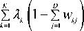
E ( C , W ) = j K ; j ( w jj Z x, e Ct ( x, — V kj )2 + rw j log w kj ) k = 1 j = 1 i k
+1l ^ (1 - iLW kj )
Besides EWKM, entropy is also taken into account in the local adaptive clustering (LAC) [17] algorithm for subspace clustering; the objective function of LAC can be expressed as:
KD
L ( C , W ) = ZZ wk
J C ( xj - V ,)2
x , ec ‘ I I —+ hw kj log wk
By comparing Eq.(2) and Eq.(3), it is found that their objective functions are very similar and the only difference is that the effect of cluster size is considered in Eq.(3) but omitted in Eq.(2).
By inspecting these soft subspace clustering techniques, it is clear that the within-cluster compactness is only considered to develop the corresponding algorithms. It is however anticipated that the performance of clustering can be further enhanced by including more discriminative information. Recently, Chen has proposed an adaptive algorithm for soft subspace clustering (ASC) [26] by taking into account both minimization of the compactness of the subspace clusters and maximization of the subspace in which the clusters exist. The objective function of ASC can be expressed as:
KD 2
A ( C , V , W ) = Z I Z Z w , ( x j - vv ) - hk x size ( Sk ) k = 1 к j = 1 x i e Ci ' 7
KD
+z л ^ Lz w j - 1
where hk is a balance parameter and size ( Sk )the size of the subspace. We can observe that ASC considers subspace information in clustering besides the within-cluster compactness which is omitted in other soft subspace clustering, however, this subspace clustering algorithm requires an additional step to obtain the adaptive parameter which increase the running time.
By inspecting the existing soft subspace clustering algorithms, the problems we find out are as follows:
-
1. Most of the existing subspace clustering techniques focus on the within-compactness and omitted the other important information of the subspace.
-
2. Require to set or spend more time to figure out the value of additional parameter.
-
3. Lack of effective initialization method to achieve a better clustering result.
B. Our contributions
The major contributions of this paper are as follows.
-
1. Unlike most existing soft subspace clustering algorithms, we proposed the concept of subspace difference to develop the within-subspace information. Both the within-cluster compactness and subspace difference are employed at the same time to develop a new optimization objective function, which is used to derive the proposed soft subspace clustering based on subspace difference (SDSC) algorithm.
-
2. We proposed an improved initialization algorithm in high dimensional space with a new density measure by considering the distribution of each point’s neighborhoods. It means the density of a point is composed of the similarity and the structure between neighbors.
-
3. The performance of the proposed SDSC algorithm was investigated using real highdimensional data, and achieved better clustering result.
-
III. The Novel Initialization Method
A. The existing initialization algorithms
Currently, cluster center initializing methods have been categorized into three major families, namely random sampling methods, distance optimization methods, and density estimation methods [21] . Random sampling methods are the most widely used methods which usually initialize cluster centers either by using randomly selected input samples, or random non-heuristic parameters. Being one of the earliest references in literature, Forgy [22] adopted uniformly random input samples as seed clusters. Distance optimization methods are proposed to optimize the inter-cluster separation. Among them, SCS [23] is a variable K-Means implemented in SAS. However, it is sensitive to both initial parameter and presentation order of inputs. Density estimation methods are based on the assumption that dataset follow Gaussian mixture distribution, which identifies the dense areas to the initial cluster centers. Algorithm KR [24] proposed by Kaufman estimates the density through pairwise distance comparison, and initializes seed clusters using input samples from areas with high local density. KR also has the drawback of huge computational complexity. As a result, it is ineffective with large datasets.
These methods are limited to huge computational complexity and presentation order of inputs. Moreover, these approaches would loss effectiveness in high dimensional space due to “curse of dimensionality” [4] and the inherently sparse data.
B. Algorithm DBNDI
Searching initial centers in high dimensional space is an interesting and important problem which is relevant for the wide various types of k-means algorithm. However, this is a very difficult problem, due to the “curse of dimensionality” and the inherently sparse data. Motivated by these problems, we propose a new algorithm DBNDI, which explores a new method to calculate the density for improving the search accuracy. We explore a novel density measure by considering the distribution of each point’s neighborhoods. It means the density of a point is composed of the similarity and the structure between neighbors. The notions of similarity and density can be describe as follows.
Definition 2 [19] .Let tNN ( p ) be the t -nearest neighbors set of p . For V q e tNN ( p ) , the similarity between p and q , is defined as:
Sim (p, q) = j0l StNN(p, q )/ t p e tNN (q) p t tNN (q)
where StNN ( p , q ) = { x|x e tNN ( p ) and x e tNN ( q )} .
StNN (p,q) is the amount of elements in StNN (p,q). Then we can assign different weights to each point according to their unique structure of neighbors. The algorithm calculates a new weight for each neighbor of a point based on the distances proportion between the point and its neighbors. Let dist(p,q)be the distance between any two points in the dataset by using traditional Euclidean distance measure[20]. The sum distance between p and its near neighbors can be measured, and it can be formally defined as:
t
D p = E dist ( p , q )
i = 1
where qi e tNN(p),i = 1,...,k .Given the influents imposed by different distances proportion of near neighbors, we assign weights wi' in the following definition.
Definition 3 .The notion of probability density of point p , named DBNDF (Distance-Based Neighborhood Density Factor), is calculated as:
NBNDF (p) = ^Tw1S1(14)
i = 1
, Dp -dist(p,qi)
where w = —----------and S = i (t -1)Dpi
Sim ( p , q i ) > 0
Sim ( p , q i ) < 0
i = 1,...,t . t is the size of near neighbor list of p , 0 is the value of similarity threshold for Sim(p,q), and qi is
the i - th nearest neighbor of p .It’s easy to
t get0 < wi < 1and ^wi = 1 to one point in high dimensional i=1
space.
To identify the similarity requires determining the value of 0 . This is a very experience-dependent process. Owing to the existing problems of high dimensional space, the number of low similarity is numerous, and the number of high similarity is relatively lack. The ideal value of parameter can filter out low similarity and distinguish the reasonable scope of similarity.
Based on these ideas, a counting-based approach is adopted to facilitate the calculation of 0 . In this approach, as for the whole pairs of the point and its neighbors, we can find all different similarities by definition 3. Let V be a vector to record the different similarities and their numbers. Then we use sum ( V ) to state the total number of all similarities and avg ( V ) as the average value of sum ( V ) . If the amount of any similarity in V gets most close to avg ( V ) , it means this element divided all similarities into two parts, the similarities of each part have approximately same amount. And the similarity of this element can be the value of 0 . Based on a large number of experiments, we find that the above rule is appropriate in most cases. Fig.2 shows the process of calculating the value of 0 .
Step1: Declare a vector V of two elements, one stores similarity, and the other represents its amount.
Step2: Filling in the vector V .
Step3: Calculate sum ( V ) .
Step4: Compute avg ( V ) .
Step5: Filter out the similarity in V which is most
-
Figure 2. The calculation of 9
After determining the parameter, Fig.3 describes the process of proposed algorithm. It is deviated from IMSND that the improved algorithm could obtain the adaptive parameter 9 according to the similarity distribution. In this wise, DBNDI is able to improve the clustering accuracy and the ability of detecting the noise.
Algorithm DBNDI
Input: dataset X = { x 1 ,x 2, x 3 ,..., x n } , the size of neighborhood t , density threshold c , and the number of clusters k
Output: cluster center set CS
Steps:
-
1. Initialization. CS = 0 .
-
2. Declare a membership matrix U of size n x t to store neighbors of each point, Fill in this matrix by using traditional Euclidean distance measure. The value in matrix is the index of each point’s neighbors.
-
3. Declare a similarity matrix W of size n x t to store the similarity of each point. Calculate all similarities using Definition 1.
-
4. Declare a parameter 9 to be similarity threshold. As mentioned in Fig.1, determine the value of similarity threshold 9 .
-
5. Based on Definition 2, count the density factor DBNDF of each data point and rank them in order.
-
6. Given the density threshold c , mark and eliminate the data points as outliers while their DBNDF values are below the threshold.
-
7. According to the order of DBNDF values generated in Step 5, points with higher density neighborhoods and lower similarity are chosen as the initial centers until the number of centers achieves k .
-
Figure 3. The process of DBNDI algorithm
While reviewing some research works on initializing cluster centers [4, 5, 7, 9], the following are typical criterions of cluster initialization algorithms:
density measure which lies in the data distribution structure so that it can avoid the curse of dimensionality.
-
(4) Immunity to the order of inputs: From the discussion in section 3.2, it is obvious that DBNDI is implemented in whole data space. However, most of the other algorithms, such as SCS [4] , limited to the order of inputs.
-
IV . Clustering Algorithm SDSC
In this section, we first introduce the notions of subspace difference, and then describe the subspace clustering algorithm SDSC.
A. Subspace difference
Soft subspace techniques have a common feature: the value of the weight is relevant to the distribution of its projection subspace [27] . It means that the more compact the data distributed, the greater the dimension weight will be. Hence, the information of the weight distribution reflects the dispersion of data points in the subspace. Taken the weight of each clusters as a data object, the greater the compactness of the weight is, the more centralized the data distributed, and the subspace is more optimal. Therefore, considering the compactness of dimension weight in the objective function will benefit the clustering process to obtain better clustering results. Unlike existing soft subspace clustering, Traditional clustering is not related to the concept of dimension weight, we assumed the weight of each dimension is equal [26] . Based on the refinement of wk 1 + wk 2 + ... + wkD = 1 , the compactness of dimensional weight can be expressed as follows:
D diff( Sk) = 2 (1 - wj )2 (4)
j = 1
Where Sk refers to the k th subspace. We could calculate diff (Sk )e [ ( D — 1 ) , ( D — 1 ) 2 / d ] using the refinement of wk 1 + wk 2 + ... + wkD = 1 , then normalize it to the range of [0, 1], and give the formal definition as follows.
Definition 1 (subspace difference): Given diff ( S k ) to represent subspace difference of the k th subspace:
diff (Sk) = D 2(1 - wj) (D -1)-D +1(5)
The new objective function is written as follows:
KD2
J(C, V, W) = 21 2 2 w (xj - v) - pk x diff (Sk) I (6) k =1 V j=1 xie Ci ' '
The first term in Eq.(6) is the within-cluster compactness, and the second term is the subspace difference. The positive parameter pk controls each dimension’s balance [26] , we can definite it as:
1 D
Pk =7.2 X jj
D j = 1
where X j = 2 x , e C k ( x j - ’ -I2-
B. Objective function
Minimization of J with the constraints forms a class of constrained nonlinear optimization problems whose solutions are unknown. The usual method toward optimization of J is to use the partial optimization for W and V. In this method, we first fix V and minimize J with respect to W. Then, we fix W and minimize J with respect to V. we use the Lagrangian multiplier technique to obtain the minimization problem:
Until || V ( p ) - V ( p -1)|| < e and ||W( p ) - W ( p -1)|| < e
KD
J,(C, V, W) §§ WjXj jj
K
- §
D
— E X x
D § k j
D
D §( 1 - w . )
-
D - 1
D + 1
KD
+ § АД § w j - 1 k = 1 \j = 1 j /
By setting gradient to J1 with respect to vj, wkj and Ak, from -J- = 0 , we obtain d vkj
v j = C § X i e C k x i .
From J1- = 0 , we obtain
8 w
w k
-------- +1.
2 § Xj
From J- = У w, - 1 = 0 , we obtain 8A k § kj ,
D
D
- § X kj
A = —— kD
.
Substituting this expression back to Eq.(9), we obtain
X j ( D - 1) 1 + D
W,. = —X----- +-- kj D 2 D
2 § X j
C. Clustering Algorithm SDSC
The SDSC algorithm that minimizes J 1 , using Eq.(8) and Eq.(10), is summarized as follows:
Algorithm SDSC
Input: dataset X = { x 1 ,x 2, x 3 ,..., x n } , the size of neighborhood t , density threshold ст , and the number of clusters k
Output: C = { C 1 , C 2,..., Ck } and W
Initialization Method: Algorithm DBNDI or Random Initialization
Let p be the number of iteration, p =0;
Denote V, W as V (0) and W (0) , respectively.
Repeat
-
1. For each center v k , and for each point xi :
-
2. p = p +1;
-
3. Using Eq.() to calculate V ( p ) ;
-
4. Using Eq.() to calculate W ( p ) ;
Set C. = ]x. k = argmin,,, ddist (v,, x, )> , k i l 1,2,..., s l i
D 2 where dist l ( v , , x , ) = J§ w j ( xj - v j ) ;
-
Figure 3.The process of SDSC algorithm
where ε is a small positive number aiming to control the algorithm process. SDSC algorithm is based on the classical framework of k -means. Unlike the other k -means type soft subspace algorithms, SDSC algorithm pays attention to the subspace difference and re-defines the iterative formula. Correspondingly, the new algorithm not only continues the convergence conditions of k -means (cluster centers converge), also focuses on the dimension weights convergence.
The SDSC algorithm is scalable to the number of dimensions and the number of objects. This is because SDSC only adds a new step to the k-means clustering process to calculate the dimension weights of each cluster. Next, we only consider the three major computational steps to analyze the runtime complexity. First, partitioning the objects, this step simply compares the summation of dist (v,,x.) = , Dw,-(x.. -v, )2 for s i jij j j—1
each object in all k clusters. Thus, the complexity for this step is O( KND ) operations. Similarly, the complexity of updating cluster centers and calculating dimension weights are all O( KND ) . If the clustering process needs p iterations to converge, the total computational complexity of this algorithm is O( KNDP ).
-
V. Experiments and Analysis
-
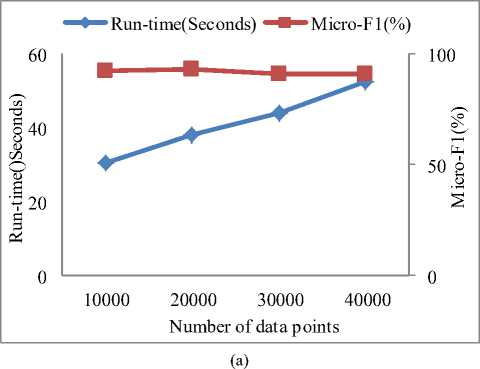
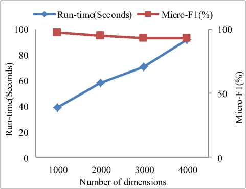
2. D 1 4 datasets validate the scalability to the number of objects. Each of them contains 4 clusters and 1000 dimensions. D 5 - 8 datasets validate the scalability to the number of dimensions. Each of them contains 4 clusters and 5000 objects.
The main purpose of this section is to verify the accuracy of our proposed SDSC algorithm. The performance of SDSC is evaluated both on real world high dimensional data and artificial data. Each dataset is normalized into a range between 0 and 1 using maxing-min normalization.
A. Datasets
In order to demonstrate the superiority of our proposed method on high dimensional data, we used five real datasets to examine the effectiveness of SDSC. The first one is Spam-Base [29] datasets is obtained from UCI Machine learning Repository. The second one is Email-1431 [30] dataset. It is an English email corpus which contains 642 normal emails and 789 spam emails. After preprocessing, each email document is mapped to a 2002dimensional vector by employing the vector space mode (VSM). The Third one is Ling-Spam [31] dataset. It contains 2412 linguist messages and 481 spam messages. We have removed low frequency words (frequency less than 0.5%) and high frequency words (frequency higher than 40%) in the preprocessing stage. Finally we have 4435 words. The last two datasets extracted from TanCorp [32], after preprocessing, we choose 1191 words, and then we have Tan-5711-1191 dataset and Tan-6301-1191 dataset. Their detailed parameters are summarized in Table 1.
To measure the scalability of SDSC to the number of dimensions and the number of objects, we generated 8 datasets based on the method suggested by Aggarwal et al [8], the detailed descriptions are summarized in Table
Table 1 . Some information about the real-world datasets
|
Datasets |
Size |
Dimension |
Cluster number |
|
|
SpamBase |
4601 |
54 |
2 |
|
|
Email-1431 |
1431 |
2002 |
2 |
|
|
Ling-Spam |
2893 |
4435 |
2 |
|
|
Tan-5711-1191 |
5711 |
1191 |
3 |
|
|
Tan-6301-1191 |
6301 |
1191 |
4 |
|
|
Table 2. Summarized parameters of the synthetic datasets |
||||
|
D 1 - 4 |
4 clusters and 1000 dimensions |
|||
|
the number of |
D 1 |
D 2 20000 |
D 3 30000 |
D 4 |
|
objects |
10000 |
40000 |
||
|
D 5 - 8 |
4 clusters and 5000 objects. |
|||
|
the number of dimensions |
D 5 |
D 6 |
D 7 |
D 8 |
|
1000 |
2000 |
3000 |
4000 |
|
B. Experiment Setup
We have implemented SDSC in C++ and all experiments were run on a PC with a 2.99GHz CPU and 2GB RAM. In order to evaluate the performance of our algorithm SDSC, we compare its performance with FWKM [16], EWKM [17] and FSC [25]. As mentioned in section 2, we explore a novel initialization method for high dimensional data. To have a better comparable results, first, like the other soft subspace algorithm, we will implement SDSC algorithm with the same initialization method (random initialization), and then we apply DBNDI technique to SDSC algorithm and the other algorithms. Three comparable algorithms all require input parameters; we specify their parameters based on the value suggested by [16], [17] and [25]. The input parameters of DBNDI are specified in Table 2.
To measure the goodness of clustering, we employ two well-known indexes Micro-F1 [27] and Macro-F1 [27] . Where F1 [27] is defined as.
_ 2 x Recall x Precision
F1 =--------------------
Recall + Precision
where recall is ratio between the number of correct positive predictions and the number of positive examples; precision is ratio between the numbers of correct positive predictions [27].
C. Experimental results on Real-World Data
According to the use of sampling or approximation techniques, the k -means type algorithms are no longer determinate and may vary with different runs of the algorithm. Hence the experiments randomly run 100 times using these methods and analyze their average accuracy.
Table 4 and Table 5 show the accuracy of four methods with the random initialization. As they show, SDSC yields better results than the competing algorithms on four datasets, in terms of both Micro-F1 and Macro-F1. We noted that the average accuracy of our proposed algorithm is almost beyond 80% which is improved while it compares to the other three techniques. As for the uneven distribution of Ling-Spam dataset, the average accuracy of the other three algorithms is almost 60%; however, SDSC continues to show advantages and achieves the clustering accuracy of 80%. To the highest dimensional dataset, Emial-1431, other clustering algorithms on average only receives the clustering precision of 70% which is given 90% using SDSC algorithm.
The comparisons results with the DBNDI algorithm are shown in table 6 and table 7. Experimental results demonstrate that the initial centers chosen by DBNDI can benefit clustering results. The obvious improvements indicate that the proposed initial algorithm is more suitable for K-Means type algorithm in high dimensional space.
As Fig.5 shows, while clustering the same dataset, the time for EWKM clustering is significantly more than other three algorithms, this is because selecting the appropriate algorithm parameters for EWKM algorithm is a timeconsuming process. The average running time of other three algorithms are almost same; however, SDSC algorithm has a better clustering accuracy in the same operating conditions.
D. Simulation Result
We conducted extensive experiments on the eight synthetic datasets, investigated the scalability of our proposed to the number of data points and the number of dimensions. The results are reported below.
Fig.6 shows the relationships between the runtime and the number of dimensions and objects, repectively. We can see that the runtime of SDSC increased linearly as the number of dimensions and objects increased. These results were consistent with the algorithm annlysis in Sction 3 and demonstrated that SDSC is scalable.
Table 3. Specified Values of Input Parameters for DBNDI
|
Datasets |
Parameter settings |
|
SpamBase |
z =50, ст =0.02 |
|
Email-1431 |
z =50, ст =0.02 |
|
Ling-Spam |
z =50, ст =0.02 |
|
Tan-5711-1191 |
z =45, ст =0.02 |
|
Tan-6301-1191 |
z =40, ст =0.025 |
Table 4. Comparison of the clustering results on the real-world datasets (Micro-F1) with the random initialization
|
SpamBase |
Email-1431 |
Ling-Spam |
Tan-5711-1191 |
Tan-6301-1191 |
|
|
SDSC |
0.7013 |
0.9257 |
0.7962 |
0.8954 |
0.8091 |
|
EWKM( γ =0.5) |
0.5673 |
0.5829 |
0.6543 |
0.5783 |
0.4984 |
|
FWKM( β =1.5) |
0.6411 |
0.6027 |
0.8402 |
0.6683 |
0.5648 |
|
FSC( α =2.1) |
0.5984 |
0.6542 |
0.6146 |
0.6428 |
0.6184 |
Table 5. Comparison of the clustering results on the real-world datasets (Miaro-F1) with the random initialization
|
SpamBase |
Email-1431 |
Ling-Spam |
Tan-5711-1191 |
Tan-6301-1191 |
|
|
SDSC |
0.8001 |
0.9146 |
0.7849 |
0.9028 |
0.8054 |
|
EWKM( γ =0.5) |
0.4192 |
0.4634 |
0.5184 |
0.4793 |
0.5012 |
|
FWKM( β =1.5) |
0.4996 |
0.4871 |
0.4957 |
0.5839 |
0.5237 |
|
FSC( α =2.1) |
0.4735 |
0.6157 |
0.4843 |
0.4918 |
0.4896 |
Table 6. Comparison of the clustering results on the real-world datasets (Micro-F1) with the DBNDI initialization
|
SpamBase |
Email-1431 |
Ling-Spam |
Tan-5711-1191 |
Tan-6301-1191 |
|
|
SDSC |
0.8123 |
0.9620 |
0.8892 |
0.9527 |
0.8956 |
|
EWKM( γ =0.5) |
0.6098 |
0.6247 |
0.7016 |
0.6234 |
0.5761 |
|
FWKM( β =1.5) |
0.6983 |
0.6672 |
0.8714 |
0.7029 |
0.6172 |
|
FSC( α =2.1) |
0.6483 |
0.7037 |
0.6749 |
0.7011 |
0.6798 |
|
Table 7. Comparison of the clustering results on the real-world datasets (Miaro-F1) with the DBNDI initialization |
|||||
|
SpamBase |
Email-1431 |
Ling-Spam |
Tan-5711-1191 |
Tan-6301-1191 |
|
|
SDSC |
0.8793 |
0.9309 |
0.8094 |
0.9164 |
0.9034 |
|
EWKM( γ =0.5) |
0.5092 |
0.5783 |
0.6035 |
0.5672 |
0.6092 |
|
FWKM( β =1.5) |
0.5004 |
0.5267 |
0.5861 |
0.6049 |
0.5984 |
|
FSC( α =2.1) |
0.5284 |
0.7035 |
0.5283 |
0.5381 |
0.5436 |
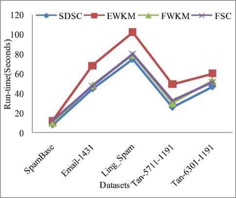
Figure 5.Comparison of the runtime of different algorithms
-
I. Conclusions and Future Work
In this paper, we have proposed a new k-means type subspace clustering algorithm, SDSC, with a novel initialization method for high dimensional sparse data. In this algorithm, we simultaneously minimize the within-cluster compactness and optimize the subspace by evaluating the subspace difference. Besides, we introduce a novel initialization method which suitable for high dimensional data, and benefit the clustering results. SDSC requires no additional input parameters. The experimental results on both synthetic and real datasets have shown that the new algorithm outperformed other k-means type algorithms, such as FWKM, EWKM and FSC. Except for clustering accuracy, the new algorithm is scalable to high dimensional data and easy to use because it has no input parameters. Future work will focus on how to develop a more effective way to specify the input parameters of our proposed initialization algorithm according to the various structure of dataset.
(b)
Figure 6.The relationships between the runtime of SDSC, and different numbers of data points and dimensions.
References An Initilization Method for Subspace Clustering Algorithm
- A. Jain, M. Murty, P. Flynn, “Data clustering: a review”, ACM Comput. Surv. 31 (1999) 264–323.
- Y. Cao, J. Wu, “Projective ART for clustering data sets in high dimensional spaces”, Neural Networks 15 (2002) 105–120.
- A. Hotho, A. Maedche, S. Staab, “Ontology-based text document clustering”, in: Proceedings of the IJCAI 2001 Workshop on Text Learning: Beyond Super- vision, 2001.
- L. Parsons, E. Haque, H. Liu, “Subspace clustering for high dimensional data: a review”, SIGKDD Explorations 6 (1) (2004) 90–105.
- R. Agrawal, J. Gehrke, D. Gunopulos, P. Raghavan, “Automatic subspace clustering of high dimensional data for data mining applications”, in: Proceedings of the ACM SIGMOD International Conference on Management of Data, 1998, pp. 94–105.
- C.H. Cheng, A.W. Fu, Y. Zhang, “Entropy-Based Subspace Clustering for Mining Numerical Data”, in: Proceedings of the Fifth ACM SIGKDD International Conference on Knowledge and Data Mining, 1999, pp. 84–93.
- S. Goil, H. Nagesh, A. Choudhary, Mafia, “efficient and scalable subspace clustering for very large data sets”, Technical Report CPDC-TR-9906-010, Northwest University, 1999 .
- C. Aggarwal, C. Procopiuc, J.L. Wolf, P.S. Yu, J.S. Park, “Fast algorithms for projected clustering”, in: Proceedings of the ACM SIGMOD International Conference on Management of Data, 1999, pp. 61–72.
- C.C. Aggarwal, P.S. Yu,” Finding generalized projected clusters in high dimensional spaces”, in: Proceedings of the ACM SIGMOD International Conference on Management of Data, 2000, pp. 70–81.
- K.G. Woo, J.H. Lee, Findit: “A fast and intelligent subspace clustering algorithm using dimension voting”, Ph.D. Dissertation, Korea Advanced Institute of Science and Technology, 2002.
- C.M. Procopiuc, M. Jones, P.K. Agarwal, T.M. Murali, “A Monte Carlo algorithm for fast projective clustering”, in: Proceedings of the ACM SIGMOD Conference on Management of Data, 2002, pp. 418–427.
- K.Y. Yip, D.W. Cheung, M.K. Ng, “A practical projected clustering algorithm”, IEEE Trans. Knowl. Data Eng. 16 (11) (2004) 1387–1397.
- K. Chakrabarti, S. Mehrotra,” Local dimensionality reduction: A new approach to indexing high dimensional spaces”, in: Proceedings of the 26th Interna- tional Conference on Very Large Data Bases, 2000, pp. 89–100.
- Z.H. Deng, k.S. Choi, F.L. Chung, S.T. Wang. “Enhanced soft subspace clustering integrating within-cluster and between-cluster information”. Pattern Recognition 43(2010) 767-781.
- G. De Soete, “Optimal variable weighting for ultrametric and additive tree clustering”, Qual. Quantity 20 (1986) 169–180.
- L. Jing, M.K. Ng, J. Xu, J.Z. Huang, “Subspace clustering of text documents with feature weighting k-means algorithm”, in: Proceedings of the Ninth Pacific-Asia Conference on Knowledge Discovery and Data Mining, 2005, pp. 802–812.
- C. Domeniconi, D. Gunopulos, S. Ma, B. Yan, M. Al-Razgan, D. Papadopoulos, “Locally adaptive metrics for clustering high dimensional data”, Data Min. Knowl. Discovery J. 14 (2007) 63–97.
- K.L. Wu, J. Yu, M.S. Yang, “A novel fuzzy clustering algorithm based on a fuzzy scatter matrix with optimality tests”, Pattern Recognition Lett. 26 (5) (2005) 639–652.
- Y. Zhang, Q. Jiang. “An Improved initialization method for clustering high-dimensional data”, the 2th International Workshop on Database Technology and Applications, 2010.
- L. Chen, Q. Jiang, L. Chen. “An initialization method for clustering high-dimensional data”, First International Workshop on Database Technology and Applications, 2009.
- He, j., Lan, M., Tan, C., Sung, S., Low, H.. “Initialization of cluster refinement algorithms: A review and comparative study”. Proceeding of the IEEE IJCNN2004.
- E. Forgy, “Cluster analysis of multivariate data: efficiency vs. interpretability of classifications”, In WNAR mretingx, Univ of ColifRiverside, number 768, 1965.
- Tou, J., Gonzalez, R.: “Pattern recognition principles”. In: Addison Wesley, Massachusetts, 1974.
- L. Kaufman and Rousseeuw. “Finding groups in data: An introduction to cluster analysis”. Wiley, New York, 1990.
- G.J. Gan, J.H. Wu, Z.J. Yang, “A fuzzy subspace algorithm for clustering high dimensional data”, in: X. Li, O. Zaiane, Z. Li (Eds.), Lecture Notes in Artificial Intelligence, vol. 4093, Springer, Berlin, 2006, pp. 271–278.
- L. Chen, G. Guo, Q. Jiang. “An adaptive algorithm for soft subspace clustering”, Journal of Software, 2010,21(10):2513-2523.
- Y. Zhang, Q. Jiang. “A k-means-based alogorithm for soft subspace clustering”, Journal of Frontiers of Computer Science and Technoloty, 2010,4(11:1019-1026).
- P., B.: “Survey of clustering data mining techniques”. In: Technical Report, Accrue Software, Inc. 2002.
- SpamBase. ftp.ics.uci.edu:pub/machine-learning-databases
- Email-1431. http://www2.imm.dtu.dk/-rem/data/
- Ling-Spam. http://www.aueb. gr/users/ion/data/
- TanCorp. http://lcc.software.ict.ac.cn/~tansongbo/corpus1.php
