Анализ прикладных моделей ионосферы для расчета распространения радиоволн и возможность их использования в интересах радиолокационных систем. I. Классификация прикладных моделей и основные требования, предъявляемые к ним в интересах радиолокационных средств

This is the first of a series of articles devoted to the critical analysis of foreign and domestic applied models of the ionosphere and to the evaluation of their use in radar systems.

Modern radars are known to work in HF, VHF, UHF, and S bands. In the first band, the so-called single-hop over-the-horizon radars have been developed and continue to be elaborated [Akimov et al., 2014; Akimov, Kalinin, 2017; Fabritsio, 2018] . The attempt to devise workable multi-hop over-the-horizon radars failed both in the USSR and in the USA. In other bands, imaging radars operate [Shield of Russia ..., 2009; Powerful horizon radars ..., 2013; Conceptual approaches ..., 2017] .

For over-the-horizon radars, the ionosphere is a radio wave propagation channel. The HF band allows us to use information from these radars to determine a number of important geophysical and radio physical characteristics of the ionosphere, which in turn makes it possible to adapt the radars to continuously varying medium parameters. An integral part of over-the-horizon radars is additional radio instruments (vertical sounding ionosondes, means of oblique and backscatter sounding, receivers of signals from global navigation satellite systems (GNSS)

GLONASS and GPS, etc.), adopted to more accurately assess ionospheric parameters at h ≤400–450 km, where HF waves propagate. The use of ionospheric models for over-the-horizon radar is determined by:

• •    approximate assessment of tactical and technical characteristics of over-the-horizon radars during their designing regarding to location and field of view;

• •    interpretation of experimental data is often uncertain;

• •    development of short-term and long-term forecasts of the ionosphere to improve the functionality of the radars [Akimov, Kalinin, 2017] .

The imaging radar situation, on the one hand, is less complicated because in this case the ionosphere is not a wave propagation channel due to an increase in the operation frequency — it is only a medium affecting the propagation. On the other hand, fields of view of the most important imaging radars of national significance are outside the territory of Russia. It therefore becomes almost impossible or very expensive to provide the required ionospheric evidence (an exception is GNSS GLONASS and GPS receivers). Moreover, the imaging radars are designed to detect and track objects at very high altitudes h , much higher than F2-region heights, as well as at large distances from the place of their location. Thus, the use

This is an open access article under the CC BY-NC-ND license

of any ionospheric models for improving the operational efficiency of the imaging radars is as important as that of the over-the-horizon radars. To the three problems, solved with the ionospheric models, for the imaging radars we should add another one [Powerful-Horizon Radar.., 2013] — real-time correction of trajectory measurements of objects (range L , elevation angle φ, velocity v ).

The consideration of the negative effect of the ionosphere on radar is a fairly complex problem due to the high variability of ionosphere parameters with increasing h as a result of decreasing air density and the presence of various types of disturbances associated primarily with solar and magnetic activities. Without dwelling on the history of the ionospheric modeling, we note only that all the models can be divided into two large classes — scientific and applied. The first one generally includes theoretical and quite complex models, a large number of physical, chemical, and dynamic processes covering a very wide range of heights (from ~90–100 km up to magnetospheric heights). Scientific models refine existing knowledge of medium or identify any new mechanisms affecting the ionosphere in the context of solar-terrestrial links (top to bottom) or lithosphere-atmosphere-ionosphere interactions (bottom to top). Applied models are used largely for predicting radio wave propagation in a wide frequency range.

In our opinion, ionospheric models for radar systems are currently selected somewhat arbitrarily, according to the shallow analysis of output parameters of the models, without criticizing the basic principles on which a model is based. General requirements for such models have not been formulated, except for some considerations made by Aksenov et al. [2017a] . The main purpose of this paper is to justify and set these requirements, which required us to develop a virtually full classification of ionospheric models and to describe modern methods of considering the medium effect on radio wave propagation for radar problem.

CLASSIFICATIONOF IONOSPHERIC MODELS

Oddly enough, there is no full classification of ionospheric models now, despite the obvious need for its development (some attempts have been made in [Becker et al., 2013; Kozlov et al., 2014, 2018; Aksenov et al., 2017a] ). This classification can be useful, for example, for setting tactical and technical requirements for ionospheric research, requirements for models, and in some other cases. The classification described below considerably refines the proposals for classification of medium models formulated in [Becker et al., 2013; Kozlov et al., 2014, 2018; Aksenov et al., 2017a] .

Ionospheric models can be classified

• 1)    according to methods of their development: theoretical, empirical, semi-empirical;

• 2)    according to approach: deterministic (static), dynamic, probabilistic and statistical;

• 3)    according to scales of space described by the model: global, regional, covering a limited region (for example, equatorial, mid-latitude, polar), and local, designed for a point or a fairly small spatial scale;

• 4)    according to the season: for winter (November, December, January, February), spring (March, April) and

fall (September, October) equinoxes, summer (May, June, July, August);

• 5)    according to the range of heights: for D-, E-, F1-, F2-regions of the ionosphere, sporadic E layer, the outer ionosphere;

• 6)    according to the time of the day: for diurnal, nocturnal, dawn and dusk period;

• 7)    according to the ionospheric parameters defined by the model: electron density N e , frequency of collisions between electrons and ionized ν ei and neutral ν en components, N e gradients in height h , latitude, and longitude, the temperature of electrons T e , ions T i , neutrals T n , ionospheric irregularities;

• 8)    according to the degree of ionospheric disturbance depending on latitude, solar and magnetic activity (solar flares, absorption in the polar cap, in the zone of the auroral oval, etc.) or on artificial effects (heating facilities, etc.) [Kozlov et al., 1988, 1990; Kozlov, Smirnova, 1992a, b; Physics of a Nuclear Explosion, 1997] ;

• 9)    according to the form of presentation of ionospheric parameters: analytical, tabular, graphic.

Many of the listed features are obviously interdependent. The applied models considered have several features, but for their classification and selection we should identify the most important.

METHODS OF CONSIDERING RADIO WAVE PROPAGATION MEDIUM

For over-the-horizon and imaging radars, methods of considering the wave propagation medium have some common features, but generally differ markedly.

Over-the-horizon radars

As have been noted [Golovin, Prostov, 2006; Akimov et al., 2014, 2017; Fabritsio, 2018] , to improve information and technical characteristics of modern over-the-horizon radars their work must be based on the principle of frequency adaptation. This means that the optimal operating HF-band frequencies should be selected depending on radio wave propagation conditions along a given path and on interference situation at a receiving site. Numerous experimental studies suggest that the frequency adaptation can significantly improve the functionality of over-the-horizon radars and predetermine the reduction in transmitter power.

The adaptation of the radar operating mode involves the following main stages:

• •    ionospheric sounding along a selected radio path at L ≤400–500 km;

• •    determination of ionospheric parameters;

• •    prediction of ionospheric parameters;

• •    adaptive control of information and technical characteristics of the radar: operating frequency, data transmission rate, transmitter power, transmitted signal type, etc.

Thus, the over-the-horizon radar requires additional tools of ionospheric diagnostics (we will not dwell on the description of these tools here), and this is the fundamental difference between over-the-horizon and imaging radars.

Ionospheric models are employed mainly during stages of design and operation of over-the-horizon radars, the requirements for the prediction of ionospheric parameters at these stages being different [Akimov, Kalinin, 2017].

When designing over-the-horizon radars, the longterm models of regular ionospheric layers are used which take into account long-term statistics, described by average characteristics of ionospheric parameters. This approach is based on recommendations of the International Telecommunication Union [Recommendations..., 2010] . They say that when evaluating medium parameters we should be intent on the procedure based on the International Reference Ionosphere (IRI) or on a more flexible procedure specific to the NeQuick model. However, the use of statistical data from deterministic models allows us to obtain only mean estimates of propagation conditions, without probabilistic features of their occurrence in different geophysical situations, thus making it impossible to assess probabilistic features of radar output. It is, therefore, better to use probabilistic and statistical models of the ionosphere at the design stage [Kozlov et al., 2014] , which can answer the question: what radar characteristics (and with what probability) occur under different space weather conditions.

Under the operation of the over-the-horizon radar, which is constructed as an adaptive system, we can employ a wider range of models (including deterministic ones) because none of the models developed answer with high probability to the question about current operating conditions. Real-time calculations with medium models require their adjustment to current measurements of propagation medium parameters. One of the fundamental requirements in this situation is real-time and correct description of the vertical profile of N e up to the height of the F2-layer maximum density with different adjustments.

As shown in [Ryabova, 1994; Agaryshev, 1995; Ryabova et al., 1997] , a model unadapted to specific propagation conditions can be used only for accurately predicting the regular component of maximum usable frequencies (MUF). This may be sufficient for radio communications, but insufficient for optimal real-time radar operation at a particular azimuth because differences between real daily MUF values and calculated ones may be as great as 50 % and greater depending on external conditions. In the long-term forecast, median standard deviations (SD) of MUF for the main radio paths 2500–6000 km are 25–40 %. As for the random component, it has been experimentally established that SD of the random component:

• •    does not exceed 100–150 kHz for quiet ionospheric conditions;

• •    does not depend on the radio path length;

• •    1.5–2 times smaller in summer than in winter, and is 6–7 % of MUF.

The real-time adjustment of the model in the main radio communication facilitates error-free reception of test messages in 84 % of cases in the daytime (08:00–20:00) and in 90 % of cases in the nighttime (20:00–08:00), whereas the long-term forecast ensures error-free reception only in 54 % of cases in the daytime and in 46 % of cases in the nighttime. When selecting a noiseproof channel, a frequency-modulated continuous wave ionosonde provided reliable communications at a level of 97 %; and when selecting a channel for the long-term forecast, at a level of only ~ 68 % [Ryabova, 2004].

Imaging radars

To take into account the effect of radio wave propagation in imaging radars, a combination of direct and indirect methods is being used now [Allen et al., 1977; Du-long, 1977; Hunt et al., 2000; Karachevtsev, 2012; Ku-riksha, Lipkin, 2013; Sokolov et al., 2012] . An element of the direct methods is the direct determination of the current total electron content (TEC) on the line of sight to GNSS GPS and GLONASS satellites through the field of view of imaging radars with subsequent adjustment of mathematical medium models from these data (indirect method).

Let us consider the merits and demerits of these methods in more detail.

Direct method. One of the promising directions for calculating TEC along the path radar–medium–object is to use data on space objects whose orbital characteristics are known with high accuracy. Among these is justified satellite data from ground laser systems, ephemeris data from GNSS satellites obtained using the GPS/GLONASS receiver located near the imaging radar. Reception of GNSS signals at different azimuths provides current information on TEC in the field of view. The analysis has shown that in the general case up to 12 GNSS satellites can simultaneously be in the radar field of view.

Estimates have shown that there is a strong non-uni-formity in the distribution of GNSS satellites over azimuth in fields of view of various radars (as an example, Figure 1 shows the distribution of the azimuthal spacing of the said satellites in the field of view of an imaging radar). Hence, the efficiency of the direct method depends on the relation between spatio-temporal satellite constellation and space-time radii of correlation between the main ionospheric parameters. Data available from the literature [Ionospheric Disturbances ..., 1971; Chernov, 2002; Blagoveshchenskii et al., 2013; Shpynev et al., 2016] on space-time correlation radii (related mainly to the F2-region) shows that in quiet conditions at middle and high latitudes the correlation radii can be: in space — from ~1000 to ~1500 km, in time — from ~40–30 to ~15 min. Under disturbed conditions, the radii decrease to ~300–200 km and ~5–3 min respectively.

The above information makes it possible to approximately determine the maximum azimuthal spacing of GNSS satellites at which the TEC values from different satellites correlate at a level of ~0.95. For example, the allowable spacing is ~15° for the 500 km correlation radius and 30° for the 1000 km correlation radius. Figure 1 indicates that approximately in 9–20 % of cases the azimuthal spacing of GNSS satellites exceeds the spatial radius of the correlation region at the level of the F-region maximum electron density; the linear interpolation is, therefore, utilized to obtain TEC between adjacent measurements.

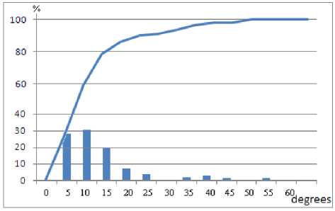
Figure 1. Integral and differential distribution of azimuthal spacing of GNSS satellites over the daily interval in the field of view of a horizon radar

Thus, GPS/GLONASS data allows us to determine medium parameters (such as TEC) in near real time along the line of sight to GNSS satellites and use them for current adjustment of the ionospheric model in hand, which is then applied to the entire field of view in order to reduce errors in satellite trajectory measurements under real cosmic background noise. However, due to the nonuniform azimuthal distribution of GNSS satellites in the radar field of view there are areas extended in azimuth with uncompensated effect of the propagation medium. The lifetime of these areas with an azimuth of 25° and more, as shown by the analysis of the azimuthal temporal staying of a GNSS satellite in the radar field of view, may be from 15 to 145 min, which in some cases exceeds the temporal radius of correlation between ionospheric parameters in the F-region. It should also be noted that there are malfunctions in the GNSS satellites during perturbations of the propagation medium (lasting from one to tens of minutes) [Kunitsyn, Padokhin, 2007; Yasyukevich et al., 2015; Pronin et al., 2019] .

TEC variations [Kunitsyn, Padokhin, 2007] are shown in Figure 2. A relative increase in TEC was ~40 TECU in ~40 min interval during the October 28, 2003 flare and ~5 TECU in a 15 min interval on November 04, 2003. We can see that there is a fairly sharp increase in TEC (the effect of a sudden increase in TEC (SITEC)).

From the maximum change in TEC in the said intervals and accepting the linear law of TEC variation, estimate the error growth in range due to TEC variations.

Using the relationship [Kolosov et al., 1969]

40.3

= f2 TEC -TEC , where f is the emission frequency, TEC0 and TECΔT is the total electron content before the disturbance and after it in the time ΔT respectively, we find that for the UHF band the error gain was ~112 m for October 28, 2003 and ~12 m for November 04, 2003; and for the VHF band for the same intervals, ~992 m and 98 m respectively. This requires a change in the information renewal rate during disturbed periods.

In recent decades, the method of forecasting the state of the ionosphere with the aid of neural networks has been ac- tively developed. These works began with attempts to develop systems for prediction of the critical frequency foF2 for a single station [Cander, 1998]. The method is based on the following assumption: since the neural network is a universal interpolator [Haykin, 1994], it is possible to train it, i.e. to find nonlinear relationships of the current state of the ionosphere with the prehistories of ionospheric characteristics and solar and geomagnetic activities and their current (or predicted) levels.

The first works in this area were based on classical feed-forward networks and multilayer perceptrons [Wintoft, Cander, 2000; Nakamura et al., 2009] . The K p , AE , F 10.7 indices for previous 24–72 hrs were commonly utilized as predictors. The forecasting horizon was 1, 6, 12, and 24 hrs. Training, test, and control data sets were selected upon the recommendations from [Haykin, 1994] . The number of layers was chosen rather arbitrarily.

Attempts have been made to build up separate networks for each month to consider the effect of seasonal variations in thermospheric parameters on the ionospheric response to geomagnetic disturbances. Nonlinear activation functions were used— sigmoidal functions or a hyperbolic tangent function [Haykin, 1994] .

Neural networks have shown a high quality of prediction of monthly median f o F2 [Cander, 1988] and a satisfactory quality of prediction of negative ionospheric storms at the hourly horizon. The prediction of ionospheric storms with a greater lead time and the prediction of positive ionospheric storms, as shown by the detailed study of the findings, were not so reliable [Wintoft, Can-der, 2000] . This is due to two separate problems. Firstly, the relative statistical weight of geomagnetically disturbed days is significantly less than that of the quiet ones. The use of all the amount of available experimental data for training leads to overtraining of the network based on geomagnetically quiet periods and poorly formed response to geomagnetic disturbances. Solar flare events are not included in the training dataset. Secondly, the use of nonlinear activation functions as the formally best for quality of the network causes a problem of multiple local minima of objective training function. There is still no single reliable method of searching for the true global minimum, and the use of an ensemble of networks leaves open the question of choosing the best option.

Understanding of these problems led to the development of neural networks based on radial basic elements [Liu et al., 2009; Huang, 2014] . Unlike feed-forward networks, the problem in this case reduces to the solution of an overdetermined system of linear equations. The use of SVD algorithms (Singular Values Decomposition) allows us to forecast ionospheric conditions with manual adjustment of the forecast accuracy. It becomes possible to obtain a rough prediction resistant to the calculation errors and a set of predictive curves (time trajectories) with different degree of detail and less resistant to variations of input data. The use of eigenvalues found by the SVD method provides a rough probabilistic estimate of the accuracy of the predicted realization. The method has shown good results in the forecast of ionospheric storms (from variations of f o F2) and TEC.

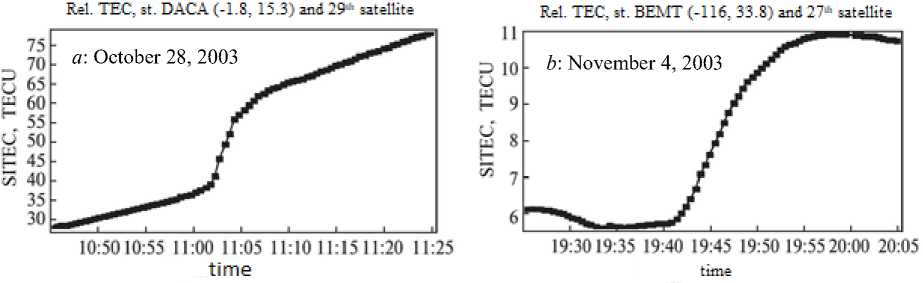
Figure 2. TEC variation for satellite – GPS receiver pairs during intense solar flares on October 28 and November 4, 2003 [Kunitsyn, Padokhin, 2007]

Recent studies have tried to exploit very promising recurrent neural networks [Boulch et al., 2018] . An additional advantage in this case is that the problem of determining the boundaries to the past in order to define the prehistory of ionospheric conditions or geomagnetic parameters is assigned to the neural network itself, thereby eliminating the subjectivity in selecting predictors and the problem of the relationship between the prehistory and the forecast horizon is solved self-consistently.

Thus, the large azimuth spacing of GNSS satellites and a sufficiently long lifetime of this spacing in the radar field of view require us to search for other approaches to solving the problem of the real-time consideration of current conditions of radar operation.

Indirect method . One of the methods able to take into account the effect of the propagation medium is the method based on radio wave propagation models, developed from geophysical models of Earth’s atmosphere and ionosphere. The medium models can describe propagation conditions throughout the radar field of view and thus solve the problem of its large size. In most cases, however, the geophysical models can estimate the mean state of the medium, which may differ significantly from the current one.

Numerous experimental data shows that, for example, at middle latitudes under absolutely quiet space weather conditions the real critical frequency f o F2 deviates from model values in over 50 % of cases. The comparison of the results of IRI-2016 N e calculations with experimental data from the DE-2 satellite at h ~250–850 km in polar and middle latitudes under different geomagnetic conditions led to the conclusion [Lyakhov et al., 2019] that only ~30 % of calculations are in the range 0±15 % of instrumental accuracy of N e satellite measurements. These examples suggest that medium models need adjusting when used for particular radars.

For this adjustment the national radar adopts quite widely current measured TEC (see above) and much less widely f o F2 [Sokolov et al., 2012] . In the latter case, it is necessary to use additional measuring instruments, which is costly; and taking into account the location of fields of view of the most important radar systems outside the territory of the Russian Federation it is practically impossible.

Thus, the mathematical medium model employed even under quiet conditions requires adjustment from current measurements of medium parameters (e.g., TEC, foF2, etc.). The integral efficiency of this approach is illustrated in Figures 3 and 4, where cumulative distribution functions of residuals over range and elevation angle are shown [Sokolov et al., 2012]. The calculations are based on UHF-radar measurements of elevation angles and ranges of tuning satellites. About 2000 individual measurements were made from March 27 to 29, 2014. Geomagnetic conditions in this period were quiet; the minimum Dst index was –22 nT.

In the first case, the cumulative distribution functions were built without compensating atmospheric errors (in Figures 3 and 4 they are designated as “Unadjusted”), i.e. actual distributions of current errors in measurements of the parameters are considered.

In the second case, corrections were introduced which were calculated by IRI-2007 from predicted Wolf numbers W , but without adjusting the model to current TEC measurements (designated as “Adjusted (forecast)”).

In the third case, we introduced corrections calculated by the ionospheric model adjusted by current measured TEC (designated as “adjusted (current)”).

The analysis of the results leads to the following conclusions:

• 1.    The introduction of corrections in the long-term forecast mode can improve the accuracy of individual measurements. Improvement in range (hereinafter for measurements designated as “Unadjusted”) is 47.6 %, in elevation angle the accuracy of individual measurements has increased to 65.4 %. A similar reduction was obtained for the SD residual. For range, SD has been improved by 43.6 %; and in elevation angle, by 37 %.

• 2.    The use of the corrections calculated in the realtime forecast mode improves the accuracy of individual radar measurements in range as compared to the longterm forecast. The resulting improvement to the mean residual in range is 82 %; and in SD, 70 %.

Approximately the same results have been obtained for the VHF radar.

Despite the encouraging conclusions, the method in hand has a significant drawback — it fits model TEC to experimental ones, using randomly varying W or F 10.7.

This could lead to absurd results from a physical point of view. If, for example, on a day the actually measured F 10.7 = 80 (low solar activity), the fit between TEC calculations and the experiment requires F 10.7 ≈ 200. Unfortunately, this situation is not discussed in the published papers. Moreover, no criteria of fit between TEC calculations and experimental data are given.

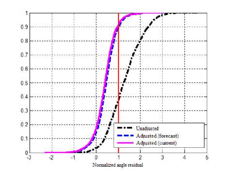
Figure 3. Cumulative distribution function for elevation angle residual

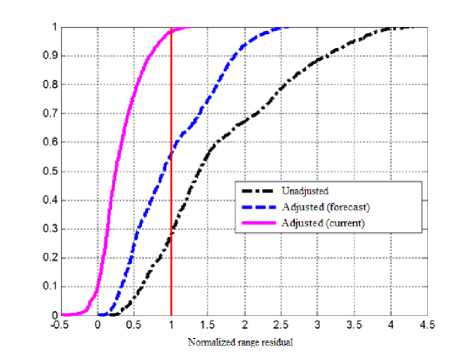
Figure 4. Cumulative distribution function for range residual

REQUIREMENTSFOR IONOSPHERIC MODELS

Considering the problems, solved with the aid of radar systems, and the geographical location of different radars (see [Aksenov et al., 2017b; wiki/Solid_State_Phased_Array_Radar_System] which schematically show the missile launch detection systems of Russia and the USA) and some technical characteristics of the stations (radiative power, wavelength, geometry of fields of view, operating modes, etc.), we formulate the requirements for the ionospheric models used in the radars:

• 1.    Height range . Medium conditions should be described at least up to 18–20 thousand km, typical of GNSS; and in the ideal case, up to the geostationary orbit.

• 2.    Latitude range . All latitudes, especially polar and middle, which are the most important for radar of the Russian Federation and the United States.

• 3.    Space weather conditions . All solar and magnetic activity levels, time of the day, seasons. Of fundamental importance is the correct assessment of the behavior of the ionosphere at all heights during various natural and artificial disturbances.

• 4.    Required medium parameters . Vertical distribution of N e ( h ), gradients of N e in latitude and longitude, effective frequencies of electron collisions with neutral com-

• ponents νen(h) and ionized components νei(h), temperatures of electrons Te(h), ions Ti(h), and neutrals T(h), concentrations of charged and neutral components.

• 5.    Ionospheric irregularities . In principle, they are included in the previous paragraph, but because of their importance for S, UHF, and VHF radars operation, we include them in a separate paragraph. Such irregularities (with different scales) at different h should be evaluated taking into account the geometry of the magnetic field in radar deployment areas.

• 6.    Assessment of conformity of the model to the main property of the ionosphere as irregular, constantly changing medium.

• 7.    Exploration of the possibility of solving probabilistic problems. Among these are: probabilities of detecting space objects, navigating, identifying parameters of areas of falling objects, etc. Solution of these problems depends not only on technical characteristics of radar and observable object, but also on the state of radio wave propagation medium.

• 8.    Performance of the model . This is a very important characteristic of the model, particularly for real-time correction of trajectory measurements.

• 9.    Verification of the model . It should be carried out primarily from experimental radiophysical data, not only from geophysical measurements, as is conventional today.

Let us make a number of comments on these requirements.

For over-the-horizon radars the upper height range should certainly be reduced to h ≈ 400–450 km. At the same time, the requirements for the quality of description of the ionosphere at lower heights rise. Of particular importance is the height region adjacent from below and from above to the F2-region maximum density whose height depends in turn on the latitude and space weather conditions.

Since the improvement of imaging radar operation is largely associated with the correct determination of TEC (see above), special attention should be given to the external ionosphere ( h ≥ 500 km). According to calculations made in [Yakim et al., 2019] , its contribution to TEC is ~15–25 %, which is not so small.

CONCLUSION

The analysis leads to the following conclusions.

• 1.    Due to the increasing requirements for radar systems, the consideration of radio wave propagation medium becomes an essential part of the development, testing, and operation of radars.

• 2.    For one-hop over-the-horizon radars working in the HF band it is possible to use additional means for diagnosing the ionosphere from signal propagation paths; for the most important imaging radars the use of such means is limited or simply impossible.

• 3.    More or less complete ionospheric models should be adopted depending on the purpose (real-time correction of trajectory measurements, interpretation of experimental radiophysical data, prediction of radar operation depending on space weather conditions and location of the stations).

• 4.    The general requirements for ionospheric models we presented here are rather rigid and can be considered as some guidelines for designers of such models.

• 5.    The problem of increasing the efficiency of the radar systems through a more correct consideration of radio wave propagation medium is extremely difficult even with the use of additional tools of ionospheric diagnostics.

We are grateful to V.V. Yakim for his assistance in preparing the manuscript. The work was carried out under State Assignment No. AAAA-A19-1190282790056-6.