Analysis of the Multi-Stage Stochastic Water Supply Recourse Model

The capability of SP in water supply systems to assess and balance various risk types is one of its main advantages. For instance, it is necessary to weigh the danger of water scarcity against the risk of poor water quality. Stochastic programming enables risk management and mitigation measures by allowing decision-makers to simulate many scenarios and evaluate outcomes under various circumstances. In multi-objective water supply systems, such as those that involve several sources of water and different uses of water, SP can also aid in the optimization of water distribution choices. Stochastic programming can assist in determining the most effective and efficient allocation techniques by quantifying the trade-offs between various objectives, like resource conservation, cost reduction, and sustainability [1-3] .

Reis, S.A.d [4] proposed a two-stage stochastic programming model featuring a fixed recourse structure for tactical planning in the soybean supply chain from the shipper's viewpoint, accounting for uncertainties related to soybean

This work is open access and licensed under the Creative Commons CC BY 4.0 License.

purchase and sale prices, external demand for soybeans, and the likelihood of crop failure. Afsana et al. [5] present a two-stage stochastic programming model to enhance farmers' decisions on land allocation for various crops. Sayma et al. [6] devised a deterministic model to assist the ready-made garments (RMG) sector in minimizing production costs and maximizing profits while optimizing resource use. Sajal Chakroborty et al. [7] devised an innovative strategy for addressing SP concerns through a decomposition-based pricing method aimed at optimizing profit in agricultural cultivation. Models with 3-stages allow for more precise control over risk management tactics. The ability of decisionmakers to manage risks and allocate resources over a variety of time periods improves their capacity to adapt to changing uncertainty[8]. Farzaneh et.al. [9] show that three-stage model give more realistic result rather than the two-stage model. To reduce transit time, transportation costs, and unmet demand, a 3-stage stochastic programming model was developed in article [10]. Secondary catastrophes often follow major disasters in real life, and their varied and unpredictable nature combined with the devastation they cause may make emergency relief efforts more difficult. For this reason, a scenario-based, 3-stage stochastic programming model is presented in [11], taking into account the relationship between primary and secondary disasters in the face of uncertainty. A three-phase stochastic programming approach has been proposed in the [12] article for inventory routing and the infrastructure building of LNG supply systems in demanding countries. Considering the opening of local distribution facilities, initial supply allocation, and last-mile relief distribution, the paper [13] proposes a 3-stage mixed-integer stochastic programming model for disaster response planning. An algorithm developed by Michael S. Casey et al. [14] generates a series of scenario trees that offer both asymptotic convergence and a measure of the first stage decision's optimality. This feature combines recourse problems with probabilistically constrained problems, two of the primary methods in stochastic programming. A new algorithm with computer code was made by Sajal Chakroborty et al. [15] to study the effects of uncertain stochastic multi-period TP problems. They developed their algorithm based on a decomposition-based pricing technique. A multiproduct, multi-period, multi-stage, and multi-site production and transportation supply chain planning challenge encountered by the textile and clothing sectors under demand uncertainty is put forth by Houssem Felfel et al. [16]. To take into account the impact of uncertainty in supply chain planning, a two-stage stochastic model is developed to address the problem. Mohammad Khairul Islam et al. [17] present four different mathematical models for optimizing and coordinating the three stages of the supply chain for Bangladeshi agricultural products. The manufacturers, retailers, and distributors were supposed to coordinate via exchanging information in this analysis. Pedro Senna et al. [18] compare a two-stage model with a multistage (or three-stage) stochastic model to optimize the biodiesel supply chain in Brazil. It was found that the flexibility of the multistage model lowers overall logistic costs when these different formulations are looked at. Shabbir Ahmed et al. [19] discuss a multi-period investment model for capacity expansion under conditions of uncertainty. They employ a scenario tree methodology to represent the progression of uncertain demand and cost parameters, alongside fixed-charge cost functions to illustrate the economies of scale in growth expenses, resulting in a multi-stage stochastic integer programming formulation for the problem. Suvrajeet Sen et al. [20] introduce models that encompass basic recourse strategies as well as more comprehensive two-stage and multistage stochastic linear programming formulations. The discussion encompasses probabilistic constraints. They examine frameworks for airline yield management, telecommunications, flood mitigation, and production scheduling. By integrating Bender’s decomposition with importance sampling, George B. Dantzig et al. [21] showed that multi-stage stochastic linear programming is the most economical way to address real-world multi-period asset allocation problem.

There is a lot of research on two-stage and multi-stage stochastic programming in different fields like agriculture, disaster management, and supply chains, but not many studies compare two-stage and three-stage models, especially in environmental infrastructure like water supply systems. Many studies either discuss theoretical ideas or focus on specific areas, but they do not look at how having more stages in a stochastic model impacts the quality of solutions and the strength of decisions when facing uncertainty. Furthermore, although some works incorporate advanced algorithmic techniques, there remains a research gap in applying and evaluating these methods within environmental systems under increasing scenario complexity. This paper aims to bridge that gap by increasing the number of scenarios and extending an existing two-stage stochastic programming model for water supply management to a three-stage model using a treebased algorithm. This method offers novel ideas about how well multi-stage SP models work, how realistic they are, and how they manage risks in environmental decision-making situations.

In this paper in section 2 an existing water supply model is presented, in section 3 analyze the existing model by capturing more sample data i.e. increasing the number of realizations, in section 4 extend the existing 2-stage SP model into 3-stage SP model by using tree algorithm, and give a comparison between the result in 2-stage and 3-stages. Finally, in section 5 give conclusion of this study.

2.    Existing Water Supply Model

A city has demand of 10 units of water. This water is supplied by an authority at no cost. But in shortage of availability of water, the authorities buy water from a company at $5 per unit. If authorities fail to meet water demand of the city, then have penalty, the city buy water from a company at $2 for the first 5 units and at $4 for the second 5 units of water. Extra amount of water of the authority realized to down-stream water with $1 per unit [22] .

In this problem the availability of water is uncertain then this problem is a stochastic programming problem. The target is to find the total minimum system cost to supply water to the city. Graphically the problem can be represented in the Fig.1. Here y 1 , y 2 , y 3 , y 4 , y 5 be the variables corresponding to the arc number of the figure. The negative sign in the objective function use for getting profit since it is a cost minimization problem.

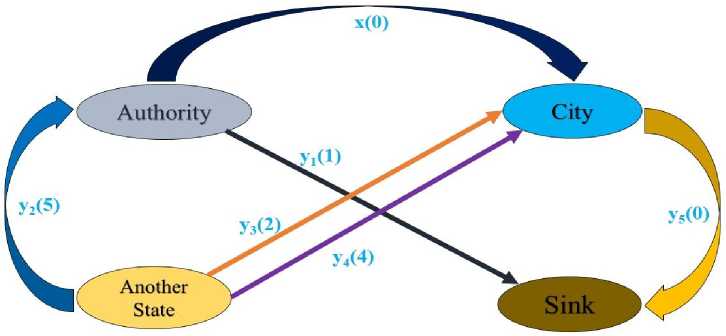
Fig. 1. Graphical network of water supply model.

• 2.1.    Solution procedure

The stochastic linear programming problems in two stages take the following form:

min: с^тх + Е [ Q ( х ( )]

X ∈ R^{n                ,}

_{․ ․}       =  ,   ≥ ⁰

Where Q(x, ^) is the optimal solution of the second-stage problem min:qTy

У ∈

S ․ t ․ Tx + Wy =ℎ, У ≥0

Here, x ∈ ℝⁿ: First-stage decision variable y ∈ ℝᵐ: Second-stage decision variable, also called recourse variable c ∈ ℝⁿ: Cost coefficients for first-stage decisions (e.g., cost per unit of production).

A ∈ ℝ^pxn: Coefficient matrix for the first-stage constraints.

b ∈ ℝᵖ: Right-hand side of first-stage constraints (e.g., resource availability).

q ∈ ℝᵐ: Cost coefficients for second-stage decisions (e.g., penalties for recourse actions).

W ∈ ℝ^mxm: Recourse matrix in the second-stage problem.

T ∈ ℝ^mxn: Coupling matrix linking first-stage and second-stage decisions.

h ∈ ℝᵐ: Right-hand side of the second-stage constraints (e.g., demand to be met).

ξ(q,h,T,W): Random variable representing uncertainty [8, 22 – 24]

Let the availability of water of the authority is 'b'. The available water amount parameter b can take value at most 12. The authority decided to provide the amount of water 'x' to reduce the total water supply system cost.

У = Flows of the water according to the arc numbers given in the Fig.1.

Since b is uncertain then to solve the problem recourse strategy is used. Let y = Flow of water in arc j and realization k. Here 5 realizations are used with equal probability 0.2. Since b is uncertain which is natural water supply, it takes value either 0,3,6,9 or 12 with equal probability 0.2. If b≤10 then x = also if b≥10 then x =10 because of the demand of the city is 10.

Then the model becomes:

min Z =∑ i ∈ I Ci Xi ⁺ p ∑∑ к ∈ _ш ^Ci ^yi^k

subject to: ∑ i _∈ I ^xi +

∑ , _e „ ^∑ . ∈ ^ =

^∑ ■ ∈ I Xi +∑   ∑ . ∈ ^ =

J ^∈ J2

^∑ , ∈ _h^∑ . ∈ ^ =

∑∑ . ∈ ^ =

J ^∈ J 4

Xi ≥0, У]к ≥0

where

C[ = first stage cost coefficient’s

X[ = first stage variables

Cj = second stage cost coefficients

Уб = second stage variables ω = different scenario’s set d =demand which is fixed

, represents upper bound and J 1 ∪ J 2=  , J 3 ∪ J 4=

For specific cost coefficients and for 5 scenarios the minimization problem becomes min z=0X+0․2

∑(- У1к +5y„ k=l

+2 Узк +4 У₄к +0 Узк )

subject to: X ⁺ У1к ^- У2к =

X ⁺ Узк ⁺ У4к ^- Узк =10

0≤ х , 0≤ У1к , У2к , Узк ≤12, 0≤ Узк , У4к ≤5, Ъ_к ∈ {0,3,6,9,12}

Where realization к = 1,․․․,5 and ^к is the availability of water supply of the authority to the city at each realization k.

Now solving the deterministic linear programming problem, equivalent to the stochastic linear programming problem using MATLAB program the minimum system cost is Z = 14․6 and X =5, the first stage decision [22].

3.    Increase the number of realizations

When there are more realizations in a stochastic programming problem, more samples from the problem's uncertain parameters are used to run the model. Scenario creation is one way that might be used to do this. By reducing the impact of sampling error and capturing a wider range of possible outcomes, increasing the number of realizations enables an improved representation of the underlying uncertainty in the circumstances. As a consequence, judgments become stronger, and risk management can be improved. However, it makes the task more computationally demanding and could call for more powerful computing resources to obtain a more realistic result.

In the water supply model only five realizations are used. Now, any number of realization n is used with equal probability. Here the uncertain parameter is b. For large n, this is a big challenge to solve this problem. In that case MATLAB program is use to solve the problem. Let p represent the possibility that each scenario will occur, then = and inc =    ,    = 0 + ( -1)∗ inc,   = 1,2 ․․․,  . Then for any number of realizations n, the water supply model becomes:

min Z=∑ i ∈ I Ci Xi ⁺ p ∑∑ к ∈ _ш ^Ci ^yi^k

subject to: ∑ i _∈ I ^i +

∑ , _e „ ^∑ . ∈ ^ =

• ^∑    ■ ∈ I Xi +∑  ∑ . ∈ ^ =

J ^∈ J2

• ^∑    , ∈ _h^∑ . ∈ ^ =

• 3.1.    Results and discussion

∑∑ . ∈ „yj* =

J ^∈ J4

Xi ≥0, У]к ≥0

Here the set ω of different realization is very large. The constraints become large exponentially with scenario number. The set of variables also become large perspective to different scenario. It is very difficult to solve the stochastic recourse problem for these large numbers of scenario and variables.

In the water supply model n is the number of realization or scenarios. A MATLAB code is developed to solve the stochastic water supply (SWS) model for any realizations, n. For different realization from 5 to 900 this MATLAB is used to find the minimum water supply cost. The objective function value corresponding to each realization is graphically shown in the Fig.2.

We note that the value of the objective function i.e. the system cost gradually decreases when the number of realizations is increase. That is, the solution becomes finer by increasing the number of realizations. This implies that by increasing the number of realizations, we capture more and more samples of the available water of the authority, our judgments become more accurate, and the feasible region of the problem becomes more accurate.

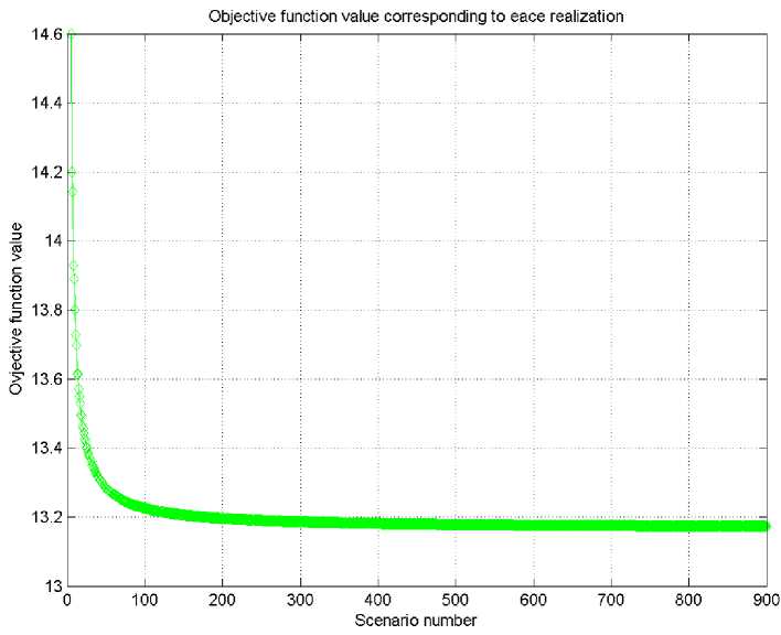
Fig. 2. Graph of objective function value.

• 4. Three-stage SWS model

• 4.1.    Introduction

• 4.2.    Model formulation

Multistage stochastic programming includes making decisions for a multistage process in the face of uncertainty. The objective of a multistage stochastic programming problem is to optimize a set of decisions across an extended time horizon. In this section, we extend the problem discussed in the previous section into three stages. At first, we expand the two-stage model to three stages graphically by using tree algorithm, considering five realizations. Then formulate the three-stage programming model from the two-stage model. Then we find out the solution of this model. We use the AMPL programming language to solve this model.

In multistage stochastic programming decisions are taken as the following pattern:

Two stage water supply recourse model

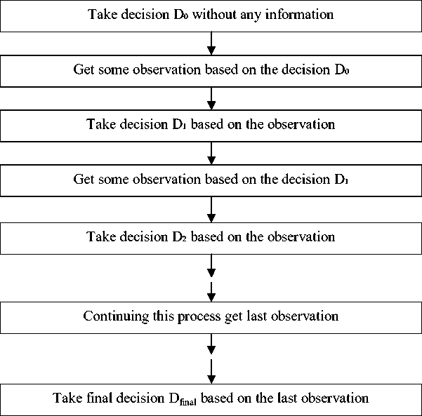
Fig. 3. Graphical network of water supply model.

The significant advantage of three-stage stochastic programming over two-stage stochastic programming is that it enables more effective decision-making in complicated and unpredictable circumstances. The present and the future are the only two time periods that are taken into account in two-stage stochastic programming. This implies that judgments are taken now without taking into account any new uncertainties or changes but rather based on predetermined future situations. The outcome might not be ideal in the long run as a result. On the other hand, three-stage stochastic programming takes into account the present, the near future, and the far future. This enables a better understanding of the risks and uncertainties that might arise in the future and provides options to modify choices as necessary. By including an additional stage, three-stage stochastic programming gives a more reliable and accurate framework that can help decision-makers make better, more informed judgments, particularly in difficult and uncertain circumstances [8,23,24].

The three stages diagram of the water supply model is shown in the Fig.4.

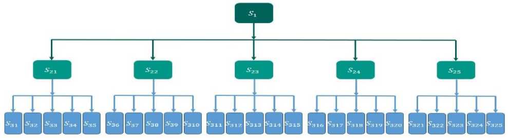
Fig. 4. Three stages water supply model diagram.

Let x 1 be the first stage decision that the authority provide water to the city, and x 2i , i=1, ..., 5 be the second stage decision that the authority provide water to the city. Then the equivalent three stage water supply problem becomes:

min ^z=∑ ■ ∈ I Ci Xi ⁺ Pl ∑      ^∑ . ∈ ^Ci ^yi^{k +} Рг ∑      ^∑ . ∈ ы^ i У jk'

J ^∈ Ji                          *—'7 ^∈ 72

subject to: ∑ i ∈ I Xi +∑    ∑ к ∈ _Miyj_k =

^∑ ■ ∈ ,Xi +∑   ∑ . ∈ _Ш1^ =

^∈ 72

^∑ ■ ∈ ,Xi +∑  ∑ . ∈ _Ш1^+∑  ∑ ^y’jk' =

*—*] ∈ /з        ¹              j -    ^-^k ∈ 0>₂

∈         ∈

• ∑^{1 ∈} iXi +∑ , ∈ „ ^∑ « ∈ ^ +∑   ∑ . ∈     =

∈ /б

• ^∑ , ∈ _h^∑ . ∈ _Ш1^ =

∑∑ . ∈ _Ш1^ = ∈ 7s

∑∑=

• / i .   *—*k^r ∈ ^2

• *—∈

∑∑=

/ i .   *—*k^r ∈ ^2

‘v ∈ Js

Where cj = first stage cost coefficient’s xi = first stage variables

Cj = second stage cost coefficients C • = third stage cost coefficients 7s = second stage variables Уб = third stage variables ω = different scenario’s set d = demand which is fixed U1, U2 represents upper bound where xi ≥0, y ≥0, y'  ≥0, y'  = third stage variable, and J-^ ∪J2 = J'2, J2 ∪J5 = J'L, J4 ∪Jg = J'2, J7∪J =

J^'_{2 .}                     jk           j k             j k

For specific values of the corresponding parameters the problem becomes min z=0Xi+(0․04×

5)∑(0X. - Рзк +5 Язк +2 ^

k=l

+4 ^S2k +0 hk )+

0․04∑(-Рзк+5Узк k=l

+2 ^r3k

+4 ^s3k +0 hk )

subject to: Х_± + P2k - 42k =   , к =1,․․․,5

^X1 ^{+ Г}2к ^{+ s}2k ^- hk =   ^, к =1,․․․,5

• * i ⁺ P₂1 ^- Я24 ⁺ ^21 ⁺ P3k ^- Язк =   ^, к =1,․․․,5

• * i ⁺ Р22 ^- Я22 ^{+ Х}22 ⁺ Рзк ^- Язк ^{=    ,} к =6,․․․,10

• * 1 ⁺ Р23 ^- Я23 ^{+ Х}23 ⁺ Рзк ^- Язк ^{=    ,} к =11,․․․,15

• ^xi + Р24 ^- Я24 + ^Х24 + Рзк ^- Язк ⁼      , к =16,․․․,20

^xi ⁺ Р25 ^- Я25 ^{+ Х}25 ⁺ Рзк ^- Язк ^{=     ,} к =21,․․․,25

^xi + Г24 + ⁵21 - ^21 + ^21 + г₃к + ^s3k - £зк =  , к =1,․․․,5

^Х1 + ^Г22 + ^S22 - ^22 + ^Х22 + Ък + ^s3k - ^Зк =  , к =6,․․․,10

^xi + ^Г23 + ^S23 - ^23 + ^Х23 + Ък + ^s3k - ^Зк =  , к =11,․․․,15

^xi + г₂₄ + ^S24 - ^24 + ^Х24 + Г₃к + ^s3k - £зк =   , к =16,․․․,20

• ^Х1 + Г₂5 + ^S25 - t25 + ^25 + Гзк + ^s3k - £зк =   , к =21,․․․,25

• 4.3.    Result and discussion

^Х1 , ^Х2к ≥0, 0≤ Р2к , Я2к , hk ≤12, 0≤ ^Г2к , ^s2k ≤5, where к =1,․․․․,5 0≤ Рзк , Язк , hk ≤12, 0≤ ^г3к , ^s3k ≤5, where к =1,․․․,25, and Ьк ∈ {0,3,6,9,12,15,18,21,24}

Here at each stage, for each realization equal probability 0.2 is used. Then the probability for each realization in the three-stage water supply model become, р = 0․2×0․2 = 0․04․

The three-stage water supply model contains a large number of variables and constraints. This is a big challenge to solve this large deterministic linear programming problem, equivalent to the three-stage stochastic linear programming problem. Using AMPL programming language we solve this three-stage problem and get the following result: The objective function value that is the system cost is z = 29.20. Solution in first stage is x 1 = 5. Second stage and third stage solutions are shown in the Table 1, and Table 2, respectively.

Table 1. Second stage recourse solution.

variable	value	variable	value	variable	value	variable	value	variable	value	variable	value
x 21	5	p 21	0	q 21	5	r 21	5	s 21	0	t 21	0
x22	5	p 22	0	q 22	2	r 22	5	s 22	0	t 22	0
x23	5	p 23	1	q 23	0	r 23	5	s 23	0	t 23	0
x 24	5	p 24	4	q 24	0	r 24	5	s 24	0	t 24	0
x25	5	p 25	7	q 25	0	r 25	5	s 24	0	t 25	0

Table 2. Third stage recourse solution.

variable	value	variable	value	variable	Value	variable	value	variable	value
p 31	0	q 31	5	r 31	5	s31	0	t 31	0
p 32	0	q 32	2	r32	5	s32	0	t 32	0
p 33	1	q 33	0	r 33	5	s 33	0	t 33	0
p 34	4	q 34	0	r 34	5	s 34	0	t 34	0
p 35	7	q 35	0	r35	5	s35	0	t 35	0
p 36	0	q 36	5	r 36	5	s 36	0	t 36	0
p 37	0	q 37	2	r37	5	s37	0	t 37	0
p 38	1	q 38	0	r38	5	s38	0	t 38	0
p 39	4	q 39	0	r39	5	s39	0	t 39	0
p 310	7	q 310	0	r310	5	s310	0	t 310	0
p 311	0	q 311	5	r311	5	s311	0	t 311	0
p 312	0	q 312	2	r312	5	s312	0	t 312	0
p 313	1	q 313	0	r313	5	s313	0	t 313	0
p 314	4	q 314	0	r314	5	s 314	0	t 314	0
p 315	7	q 315	0	r315	5	s315	0	t 315	0
p 316	0	q 316	5	r316	5	s 316	0	t 316	0
p 317	0	q 317	2	r317	5	s317	0	t 317	0

p 318	1	q 318	0	r318	5	s 318	0	t 318	0
p 319	4	q 319	0	r319	5	s 319	0	t 319	0
p 320	7	q 320	0	r 320	5	s 320	0	t 320	0
p 321	0	q 321	5	r321	5	s 321	0	t 321	0
p 322	0	q 322	2	r 322	5	s 322	0	t 322	0
p 323	1	q 323	0	r 323	5	s 323	0	t 323	0
p 324	4	q 324	0	r324	5	s 324	0	t 324	0
p 325	7	q 325	0	r325	5	s 325	0	t 325	0

But by using two stage recourse problems, the minimum cost for three stages is 2 × 14.6 = 29.20. In both 2-stage and 3-stage the total water supply system cost is same. In this SWS model one parameter is uncertain. After one stage the parameter become known, for this reason there is no impact of the 3-stage model. In that case we can propose a conjecture which is as follows:

• 4.3.1.    Conjecture:

• 4.4.    SWS model when demand and availability of water are uncertain

In stochastic model, if the number of uncertain parameters is n, then there is no impact of the (n+2) stage or more stage on the (n+1) stage of the model.

N.B. when the number of stages increase, the decision becomes more accurate. But for n uncertain parameter the decision improves up to (n+1) stage. After (n+1) stage the decision cannot improve.

In the previous case we consider that the parameter ‘availability of water’ only uncertain. In that case we get same water supply cost though the 3-stage model is more realistic rather than the 2-stage model [9,18]. Now we consider the case that the parameters demand and availability of water are uncertain. The water supply authority can collect maximum 12 units of water. So here we consider 3 cases. Which is average of water demand at each scenario is exactly 12, less than 12 and greater than 12. When demands for each scenario are [10, 11, 12, 13, 14] the water supply cost is 42.36 in 3-stage and in 2 stages the cost is 43.2. When demands for each scenario are [7, 8, 9, 10, 11] the water supply cost is 25.12 in 3-stage and in 2 stages the cost is also 26. When demands for each scenario are [13, 14, 15, 16, 17] the water supply cost is 63.32 in 3-stage and in 2 stages the cost is also 63.6. We get 1.94%, 3.38%, 0.44% batter result using 3-stage SWS model compare to 2-stage SWS model for these 3 cases respectively. The result graphically shown in the Fig.5.

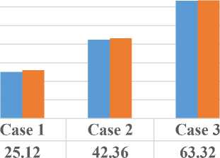
26         43.2        63.6

Й      40

8      30

I ■ 3-stage cost

I ■ 2-stage cost

Fig. 5. Cost comparison between 3-stage and 2-stage.

5.    Conclusions

The decision in stochastic optimization model is more realistic compare to deterministic optimization model. In stochastic optimization model by capturing more sample data of the uncertain parameter, the decision becomes more realistic but solve the model in this case is a very big challenge. In this paper a general MATLAB code is developed. Using this MATLAB code, we can solve the stochastic model for any number of realizations. When the number of realizations is increased the water supply system cost is decreased. In SWS model only one parameter was uncertain. So, extending to the 3-stage stochastic optimization model, the water supply system cost was not improved. Because after first stage, the uncertain parameter becomes known and based on the observation the second stage decision taken. There was no more uncertain parameter so that this becomes known in the second stage and third stage decision is taken. Based on the observation we proposed a conjecture that ‘In stochastic model, if the number of uncertain parameters is n, then there is no impact of the (n+2) stage or more stage on the (n+1) stage of the model’. Finally, we see that when we consider 2 parameters uncertain then 3-stage SWS model give better result compare to the 2-stage SWS model.

All the Declarations and StatementsAuthor Contributions Statement

Md. Asaduzzaman – Conceptualization, Methodology, Software, Writing – original draft.

Nazrul Islam – Data curation, Investigation, Visualization, Project administration.

All authors have read and agreed to the published version of the manuscript.

Conflict of Interest Statement

The authors declare no conflicts of interest.

Funding Declaration

This research received no external funding.

Data Availability Statement

The data used in this study are generated through scenario‑based simulations. The datasets and MATLAB/AMPL codes are available from the corresponding author upon reasonable request.

Ethical Declarations

Not applicable. This study does not involve human subjects or animal experiments.

Acknowledgments

None.

Declaration of Generative AI in Scholarly Writing

During the preparation of this work, the authors did not use any generative AI or AI‑assisted technologies.

Abbreviations

The following abbreviations are used in this manuscript:

SP - Stochastic Programming

SWS - Stochastic Water Supply

RMG - Ready‑Made Garments

LNG - Liquefied Natural Gas

AMPL - A Mathematical Programming Language