Application of SQL RAT Translation

Published Online August 2011 in MECS

We have already provided an object-oriented means to describe the relational algebra tree (RAT) parsed from the SQL statement. Since an intuitive solution has been found, why couldn’t we delve into its usage and explore more flexible variation adapted for different scenarios.

Reverse Query Processing (RQP) [5], a tool generating databases for testing database applications, helps to eliminate the daunting task of manual tester. An extension of RQP is RMP [3] – Reverse Manipulate Processing. It can be used for all the data manipulating statements in SQL which provides an integrated measure to execute stored-process unit testing automatically. It is wise to find a way to depict the interim result of each processing stage, hence that’s why we discuss the object-oriented way here for their possible applications.

• II.    Solutions

• A.    Previous work

Our work on the SQL’s translating into relational algebra tree can be found in [1] and we have chosen an object-oriented way to depict the translating results. We dev-ided the translating issue into 5 separate parts according to their query type. Each query type is specified with detailed example(s).

The [3] has extended the RQP algorithm to RMP. The RMP helps us to resolve the limitation of RQP and its Evaluator can translate the ‘DELETE’, ‘INSERT’ and ‘UPDATE’ manipulation into ‘SELECT’ statement with added predicate constraint(s). Therefore, our Relational

Algebra Tree should be adjusted to Reverse Relational Algebra Tree (RRA Tree) and also relationships between classes in the SQL parser should be revised in order to run the procedure more smoothly. Note that some other literatures use the “Query Tree” term so as to depict the query order more conveniently with mathematic symbols or notations.

• B.    RMP Architecture

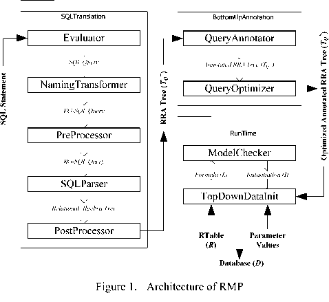
The architecture of our RMP system is shown in Fig. 1. It combines the entire architecture of the relational algebra translator with the RQP architecture supplemented with an Evaluator. The following sections will respectively explain every key stage in detail.

• C.    RMP Evaluating Algorithm

In reference [3], the evaluation of DELETE, UPDATE and INSERT statements have been discussed and verified. In order to adjust the evaluation to the naming process, we should discuss the evaluating algorithm first. The algorithm is presented in Table I.

We need to replace the DELETE, UPDATE and INSERT keywords with customized ones which can be mat- ched by our new SQL restricted grammar and recognized by the SQL parser. In the parsing stage, we also need to denote a new field in the Query class which can reflect its deviation.

TABLE I. RMP Evaluating Algorithm function evaluate (sql: SQLStatement): string var resultStr: string;

begin case getFirstToken(sql) of

DELETE :

appendToken(resultStr, DEL_SLT);

appendToken ( resultStr , ASTERISK );

append ( resultStr , sql );

INSERT :

appendToken ( resultStr , INS_SLT );

appendToken ( resultStr , INTO );

if isDefaultTuples(sql) is TRUE then appendRelaAttr(resultStr, scanTuplesFromValues(sql));

else if isPartialTuples(sql) is TRUE then appendRelaAttr(resultStr, scanTuplesFromRelaList(sql));

else appendRelaAttr (resultStr, scanTuplesFromRelaList (sql));

end if appendToken(resultStr, VALUES);

while hasValues(sql) do appendValues (resultStr, getValues (sql));

end while

UPDATE :

setStatementType ( sql , SELECT );

appendToken ( resultStr , UPD_SLT );

appendString ( resultStr , remove ( evaluate ( sql ), SELECT ));

setStatementType ( sql , DELETE );

appendString ( resultStr , evaluate ( sql ));

setStatementType ( sql , INSERT );

appendString ( resultStr , evaluate ( sql ));

SELECT :

appendString ( resultStr , toString ( sql ));

end case ;

return resultStr ;

end evaluate upper-case items denote the keywords in the SQL grammar

• D.    Revised SQL Grammar

Because we need to include the DELETE, UPDATE and INSERT statement for our new RMP system, the origin EBNF [6] grammar should be revised so as to recognize all the SQL manipulations. The new restricted grammars are shown in Table II.

TABLE II.    Revised SQL Restricted Grammar

1	query	→	gb_query | ngb_query
2	ngb_query	→	unary_query | binary_query | LPARAN unary_query RPARAN
3	unary_query	→	simple_query | exists_query | complex_query
4	simple_query	→	SELECT selector FROM relation_list [ WHERE simple_predicate ]
5	del_simple_query	→	DEL_SLT selector FROM relation_list [ WHERE simple_predicate ]
6	ins_simple_query	→	INS_SLT selector FROM relation_list [ WHERE simple_predicate ]
7	upd_simple_query	→	UPD_SLT selector

FROM relation_list [ WHERE simple_predicate ] 8 gb_query → unary_query GROUP BY gb_attr [ HAVING hav_condition ] 9 exists_query → SELECT selector FROM relation_list WHERE exists_predicate 10 del_exists_query → DEL_SLT selector FROM relation_list WHERE exists_predicate 11 ins_exists_query → INS_SLT selector FROM relation_list WHERE exists_predicate 12 upd_exists_query → UPD_SLT selector FROM relation_list WHERE exists_predicate 13 complex_query → SELECT selector FROM relation_list WHERE left_term comp_op ngb_query 14 del_complex_query → DEL_SLT selector FROM relation_list WHERE left_term comp_op ngb_query 15 ins_complex_query → INS_SLT selector FROM relation_list WHERE left_term comp_op ngb_query 16 upd_complex_query → UPD_SLT selector FROM relation_list WHERE left_term comp_op ngb_query 17 binary_query → ngb_query set_op ngb_query 18 relation_list → ID relation_list | COMMA relation_list | ε 19 gb_attr → attribute_spec_list 20 hav_condition → function_spec comp_op constant | function_spec comp_op ngb_query 21 selector → attribute_spec_list 22 attribute_spec_list → attribute_spec_list COMMA attribute_spec | attribute_spec 23 function_spec_list → function_spec_list COMMA function_spec | function_spec 24 simple_predicate → LPARAN simple_predicate boolean simple_predicate RPARAN | attribute_spec comp_op attribute_spec | attribute_spec comp_op constant 25 exists_predicate → EXISTS ngb_query 26 left_term → attribute_spec | constant 27 function_spec → ID LPARAN attribute_spec_list RPARAN 28 attribute_spec → ID DOT ID 29 Boolean → AND | OR 30 set_op → UNION | MINUS | INTERSECT 31 comp_op → EQ | NOTEQ | LT | LTEQ | GT | GTEQ 32 constant → NUM | STRING upper-case items denote the tokens recognized by SQL scanner

We have omitted the revised extended SQL grammar in order to save pages. But we should be aware of the new tokens generated by RMP evaluator which should be reflected to new extended grammar. Grammar , , , ,

, , , , , and should be appended with duplicated items with ‘ins_’, ‘del_’ and ‘upd_’ prefix and customized first token like the item 5,6,7 in Table II.

• E.    Naming Transformation and Preprocessing

In reference [2], the objective of naming transformation is to eliminate SQL ambiguous syntax problem and put the input into a form that can be accepted by the extended grammar.

In the first case, the process is alternative according to different application. In RMP, it is unnecessary to distinguish different instances of the same base relation. In the second case and also the third case, the extension of attribute names and variables eliminated are required.

Next stage, the preprocessing, includes two key steps. The first step is that rewriting the asterisk with relationattribute pairs corresponding to the closure of all its subquery. We have no idea about how the database schema is, so relations are required to be included in the input if ASTERISK is an allowed keyword. In RQP and so as the RMP, the input SQL statement is used to compare with the database schema input at runtime. In order to prevent extra conflict judging we have omitted the ‘*’ keyword. The second step is that transforming the non-base query into Group-by Query, Binary Query, Complex Query, Simple Query and Exists Query. The entire transformation discussion can be found in [2].

• F.    Parsing SQL into RA Tree and Postprocessing

In order to distinguish different Query types we need to add a new field – RMPType to the Query class definition. It is an enumeration type which is used for depicting its origin SQL statement type before evaluation. The Query hierarchy is shown in Fig. 2.

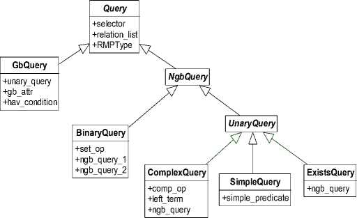
Figure 2. Hierarchy of SQL.

There are five base Query type generated from the postprocessing stage. The class diagrams of each type are shown in Fig. 3, Fig. 4, Fig. 5, Fig. 6 and Fig.7 respectively. Except for the RMPType field there is no big difference from the ones in [1]. The following chapters will discuss each Query type corresponding to its object-oriented representation of the node of Relational Algebra

Tree and the postprocessing stage related to its final output – Reverse Relational Algebra Tree.

The tree nodes in the RRA Tree should be distinguished from the RA Tree node. The Reverse Relational Algebra (RRA) is a reverse variant of the traditional relational algebra and depicted by symbol (operator) marked as op^-1 [3].

• 1)    Simple Query

Fig. 3 denotes the classes and their relationships in Simple Query . From the association between class FunctionSpec and class Function , we can figure out that the function field of FunctionSpec is nullable. When it is null, the instance denotes a group of attributes without any function applied, i.e., the attributes in projection item “PJ[S.A, S.B]”. On the contrary, the attributes are aggregated by a specific function, i.e., “SUM(S.A, S.B)” in projection item “PJ[SUM(S.A, S.B), S.C]”.

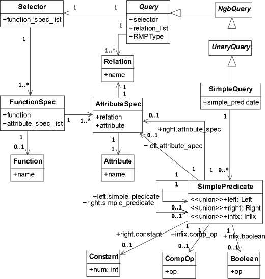
Figure 3. Class Diagram for Simple Query.

Especially, the fields in class SimplePredicate are of union type. According to the grammar < simple_pre - dicate >, we recognize that the combination of its fields can be { simple_predicate , boolean , simple_predicate }, { attribute_spec , comp_op , attribute_spec } and { attrib-ute_spec , comp_op , constant }. Therefore, there are two possible kinds of attribute for field left in class SimplePredicate , three possible kinds of attribute for the field right and two possibilities for the field infix .

There are two possible scenarios in the translation. The first one is that the simple_predicate item is empty and there is no other “external” relation. Another one is that simple_predicate occurs, which involves further calculation of “external” relations in order to incorporate them in the Cartesian product.

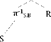
In the first case, we assume that the input string generated through the first three stages in SQLTranslation is:

SELECT F(R.A), S.B, T.C FROM R, S, T           (1)

The SQL was translated into RRA Tree whose structure is shown in Fig. 4.

Just like the Cartesian product, the θ-join is a binary operator. It connects two relations with specific predicate. As a matter of fact, until being optimized the θ-join node would never contain any predicate because it originally represents the Cartesian product between two expressions. After obtaining the Cartesian product of these three relations, the aggregation node and then the projection node are constructed upon this binary tree. The top-down sequence of these nodes is consistent with that of the SQL translation algorithm [1].

We should notice that four cases of Group-by Query should be distinguished. The first one is that the GROUP-BY clause has no effect. The second one is that there is no HAVING clause but the aggregate function should be evaluated. The third one and the fourth one are distinguished by the condition whether the HAVING clause has a nesting query or not. Except the first case, the unary query in group-by query should be changed into a form that its projection should incorporate all the attributes of its relations list order to correctly evaluate the functions.

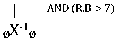
The first case is simple and when we input the following query we get the relational algebra tree shown in Fig. 7.

SELECT R.A FROM R WHERE R.B > 7 (3) AND R.C = ‘Tom James’ GROUP BY R.C

π ^{‐ 1} S.A, S.B

_∅ Χ ‐1_∅

-1

X ‐1∅

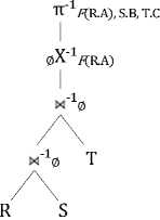
Figure 4. RRA Tree for Simple Query, Case 1.

π ‐1 F (R.A), R.C, S.A, S.B

σ ^{‐ 1} R.B = S.A

S.A, S.B Χ ^{‐ 1} F (R.A)

R

-1

XI ‐1∅

S

Figure 5. RRA Tree for Simple Query, Case 2.

In the second case, we need to assume that some relations in this query have appeared in upper level. So, we can embed this simple query into another kind of query:

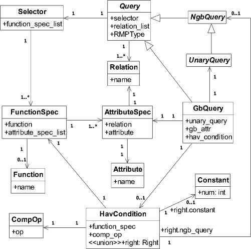
Figure 6. Class Diagram for Group-by Query.

SELECT S.A, S.B FROM S WHERE EXISTS (2) SELECT R.C, F(R.A) FROM R WHERE R.B = S.A.

Fig 5 is its corresponding relational algebra tree. Attribute ‘ S.A’ and attribute ‘ S.B’ are the “external” attributes extracted from the upper level Exists Query . They group the tuples of Cartesian product of ‘ S’ with ‘ Q’ by different values of the tuples of S and the results are manipulated by the aggregate function ‘ F’ .

2) Group-by Query

Fig. 6 is the class diagram of the group-by query. We use the class HavCondition to represent the predicate of Group-by Query . There are two possible kinds of combinations of its fields. They are { function_spec , comp_op , constant } and { function_spec , comp_op , ngb_query }. Because the first two fields of them are the same, we just need a union type to represent the third field of class HavCondition .

If the third field is a non- Group-by-Query , it means that we have to deal with an unknown nesting query. Because the class NgbQuery is an abstract class, we can utilize the polymorphism of object-oriented language for solving the nesting query problem.

тг^л

^ (R.C - 'Tom James')

‐1 π F (R.A)

R.B Χ F (R.A)

-1

XI 1∅

π ^‐1R.A, R.B, R.C

σ ^‐1R.C = 7

_∅ Χ ‐1_∅

R

1∅

Figure 7. RRA Tree for Group-by Query, Case 1.

Figure 8. RRA Tree for Group-by Query, Case 2.

In the second case, projection items of the unary_query field in the group-by query should be rewritten by incorporating all the attributes of the relations_list and we have used a table to record the relation-attribute pairs

occurred in the query while constructing the syntax tree. For instance:

culated by method connect [2] and the “external” relations are obtained by method other [2]. For instance,

SELECT F(R.A) FROM R

WHERE R.C = 7 GROUP BY R.B

SELECT R.A FROM R WHERE              (7)

EXISTS SELECT S.A FROM S WHERE S.B > 7

is translated into a relational algebra tree shown in Fig. 8.

In the third case, we need to evaluate the aggregate function in the HAVING clause and incorporate them with that of the term unary_query . For instance,

SELECT F1(R.A) FROM R WHERE R.C = 7      (5)

GROUP BY R.B HAVING F2(R.C) > 2

is translated into a relational algebra tree shown in Fig. 9. Function F1 and F2 apply to the tuples grouped by attribute R.B .

In the fourth case, we need to evaluate the nesting query in the HAVING clause. We embedded a simple query into the group-by query as the following example:

is translated into a relational algebra tree shown in Fig. 12. In order to keep the integrity of the relational algebra tree we retain the aggregation node which has no effect and this will be eliminated in the postprocessing.

The second case is that these two fields are related. From the example below, the relation set calculated by method connect is {R} and the attribute set obtained from method other is empty.

SELECT R.A FROM R WHERE EXISTS (8) SELECT S.A FROM S WHERE S.B = R.A

SELECT F1(R.A) FROM R WHERE R.C = 7      (6)

GROUP BY R.B

HAVING F2(R.C) > SELECT S.C FROM S.

So, the term ngb_query has already dealt with all the relations involved in this query and there is no “external” relation. We can perceive this effect through Fig. 13.

TT^CRA)

O"X/2(R.C) > 2

R.bX^-1 fl(U), 72(R.C)

M'X0

n"XRA, R.B, R.C

C^^XRC = 7

0Х"Х0

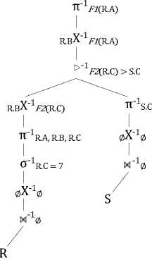
Figure 10. RRA Tree for Group-by Query, Case 4.

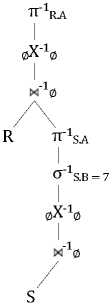
Figure 12. RRA Tree for Exists Query, Case 1.

π ^{‐ 1} R.A

_∅ Χ ‐1_∅

X ‐1∅

π ¹ S.A, R.A, R.B

σ ^{‐ 1} S.B = R.A

_∅ Χ ‐1_∅ M ‐1_∅

SR

Figure 13. RRA Tree for Exists Query, Case 2.

Figure 9. RRA Tree for Group-by Query, Case 3.

Its relational algebra tree is shown in Fig. 10. Two subqueries are linked by a semi-join with a predicate, ‘ F2(R.C) > S.C’ , extracted from the HAVING clause. In addition, this semi-join can be transformed into a θ-join following with a projection on its left term.

3) Exists Query

The class diagram that describes the Exists Query is shown in Fig. 11. The key task is to interpret the term ngb_query .

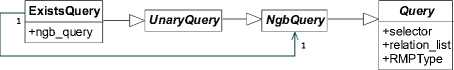
Figure 11. Class Diagram for Exists Query.

4) Complex Query

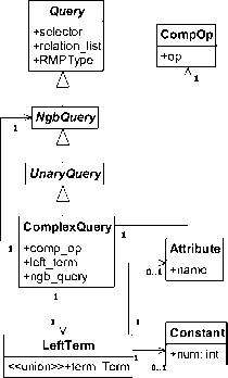
Figure 14. Class Diagram for Complex Query.

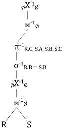
Figure 15. RRA Tree for Complex Query.

Exists Query should be discussed in two cases. The first case is that there is no connection between the field ngb_query and the field relation_list in the class Exis-tsQuery . Whether there is common relation or not is cal-

The class diagram is shown in Fig. 14. The complexquery contains a comparison between a left_term and a nesting non- Group-by-Query . Being somewhat alike the Exists Query , Complex Query , it uses the connect [2] method to calculate the common relations and the other

[2] method to obtain the “external” attributes list and then translate the comparison into a selection operation. We use the following example to reflect this effect:

the style in Fig. 18. Some redundant nodes are removed but the format of the connecting line in previous diagram is retained so as to reflect its change more clearly.

SELECT S.A FROM S WHERE S.C =           (9)

SELECT R.C FROM R WHERE R.B = S.B.

Fig. 15 is the translation result and from this we can recognize that relation ‘ S ’ is the connecting relation. The sub-query has involved all the relations in this query and the upper query just need to apply the selection ‘ S.C = R.C ’ on that expression.

5) Binary Query

A Binary Query should be translated into two subqueries linked by a binary operator (INTERSECT, UNION, or DIFFERENCE) and its descriptive class diagram is shown in Fig. 16. The Binary Query translation requires the sub-query to be associated with “external” attributes calculated by method other [2] respectively in order to become useful for upper level queries. For example,

S

π ^{‐ 1} R.A

π ^{‐ 1} T.B, R.A, R.C

π S.B

R

S

π ‐1_S.B

σ ^{‐ 1} T.C = R.C

T

x ‐1∅

R

Figure 18. RRA Tree in Fig. 17 after Reducing the Difference Operation

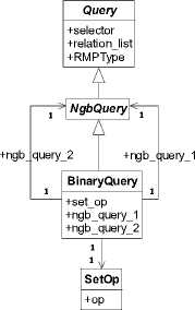
Figure 16. Class Diagram for Binary Query.

π ^‐1R.A

_∅ Χ ‐1_∅

∩ ^‐1

X^‐1∅            π ^‐1T.B, R.A, R.C

π ^‐1S.B      R σ ^‐1T.C = R.C

_∅ Χ ‐1_{∅              ∅} Χ ‐1_∅

X ‐1∅                X ‐1∅

S    TR

Figure 17. RRA Tree for Binary Query.

SELECT R.A FROM R WHERE EXISTS (10) (SELECT S.B FROM S INTERSECT

SELECT T.B FROM T WHERE T.C = R.C)

is translated into a relational algebra tree shown in Fig. 17. The “external” attribute set of sub-query ‘ SELECT S.B FROM S ’ is empty and the “external” attribute set of subquery ‘ SELECT T.B FROM T WHERE T.C = R.C’ is { R.A , R.C }. From the “external” attributes sets, we notice that the first sub-query lacks of relation ‘ R’ which is required in order to perform the intersection with the second sub-query. Hence an additional Cartesian product of the first sub-query with ‘ R’ is required.

6) Postprocessing

Except for the post-processing in [2], here we need to eliminate the tree nodes which have no effect on the expression, such as aggregation node missing the aggregate attribute, θ-join node linking only one expression without predicate or selection node missing predicate.

In RQP, the intersection operation is not allowed. So, we need find another way to transform the intersection node to equivalent mutation. Because operation ‘ A ∩ B ’ is equal to ‘ A - (A - B) ’, Difference Operator can sub-titute the intersection operation in RQP algorithm. The-efore, the RRA Tree in Fig. 17 can be transformed into

The semi-join node also needs to be transformed to a θ-join format. The semi-join can be expressed by a θ-join followed with projection onto the left term:

А В = л _A(A N В)         (11)

The transformation result of the RRA Tree in Fig. 10 ( Group-by Query , case 4) is shown in Fig. 19.

π ^{‐ 1} Fl (R.A)

R.B Χ ^{‐ 1} Fl (R.A)

I

π ^{‐ 1} R.A, R.B, R.C, Fz (R.C)

‐1

X : Fz (R.C) > S.C

R.B Χ ^{‐ 1} Fz (R.C)               π ^{‐ 1} S.C

I          /

π ^{‐ 1} R.A, R.B, R.C S

σ ^{‐ 1} R.C = 7

R

Figure 19. RRA Tree in Fig. 17 after Reducing the Semi-join.

π ‐1_R.A

TR

Figure 20. RRA Tree in Fig. 17 after Reducing the Difference Operation

At last, and perhaps the most complicated transforation, we need to detect the comparison in selection node. If the predicate is a comparison between the attribute in left term (left child of the node) and the one in right term

(right child), then the predicate in the selection node should be added to the θ-join. This is for optimizing. The RRA Tree can be simplified and we should “remove” the θ-join without predicate for it is a common situation as we can see in the example through the five type of Query . We can look back to the example in Fig. 18. The sub-tree of the Difference Operation node ‘ － ^-1’ which begins with a ‘π^-1’ node can be transformed to a new style shown in Fig. 21.

π ‐1_R.A

- ^-1

X ‐1∅

и ‐1∅

π‐1T.B, R.A, R.C и T.C = R.C

π ^‐1S.B      R

Figure 21. RRA Tree in Fig. 18 after Reducing the Empty θ-join.

• G.    Annotation and Traversal

Every node in the RRA Tree should have a reference of the Query parsed by the SQLParser for obtaining the attributes in the syntax tree structure. The node also has its own instance of RQP processing data structure for the bottom-up annotation and later processing. In the annotation stage, the Annotator (see the QueryAnnotator module in Fig. 1) will process each operator in RRA Tree generating input schema computed and extracted from the given output schema(s). Each operator should check the correctness of the input and ensure that it has generated valid output data. The detailed algorithm and computation can be found in Chapter 5 of [5].

In order to illustrate a comprehensive annotation for a specific RRA Tree, we have cited the database schemas ‘Line-item’ and ‘Orders’ (which could also be found in [5] as an illustrative example) as the input parameters. They can be expressed by the following DDL forms.

CREATE TABLE Lineitem (                  (12)

lid INTEGER PRIMARY KEY, name VARCHAR(20), price FLOAT, discount FLOAT

CHECK (1 >= discount >= 0), l_oid INTEGER);

CREATE TABLE Orders(                    (13)

oid INTEGER PRIMARY KEY, orderdate DATE);

Also, a Group-by Query is employed to help establish a RRA tree. The translation of the following query is like that one of (5) whose RRA tree structure can help us to understand the relationship of each operator:

SELECT SUM(price)                         (14)

FROM Lineitem, Orders

WHERE l_oid = oid

GROUP BY orderdate

HAVING AVG(price) <= 100;

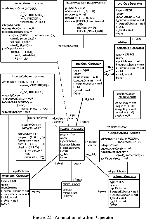
The RRA Tree should be traversed in a post-order. Firstly, the two leaf nodes in the RRA Tree is annotated with (12) and (13) setting the operation type to LEAF. Their input-Schema fields are regarded as the outputSchema of their upper node – Join Operation. Then a series of computation of constraints and dependencies should be carried out (interested reader can refer to Section 5.1 in [5]) and the new inputSchema can be passed onto its father node. In this way, the annotation continues until it reaches the root node. Fig. 21 has shown us a snap of the annotating process of the Join Operator with inputs of Lineitem and Orders . Their DDL schemas have been translated into objects instantiated through syntax recognition. Objects are represented with rectangles in Fig. 21. Those highlighted with bold and wider lines are our RRA Tree nodes.

The ensuing processing stages of RQP/RMP are straightforward: reversal in-order traversal of the RRA Tree applying the top-down data initiation algorithm (with model checking when needed). The entire descriptive algorithm can be found in [5]. It is not necessary for us to illustrate this process again here. Similar object representation method can be derived from our annotation illustration (see Fig. 22). Note that each stage, either the annotation or data initiation, should focus on the SQL parsing outcome for our RRA Tree representation discussed in Section F has been used as a frame of reference.

The Optimizer functions after the Annotator. From RRA Tree perspective, it adjusts the structure pursuing lower cost. In some way this is like the postprocessing in parsing SQL. Since existing optimizing description [5] and our former transmutation have been discussed, it is redundant to present this issue again.

The RQP/RMP system ends up outputting the final database instance with specific form depending on what the experimenter wants to get at. The generated database instances have been stored in MySQL 5.0 database management system in our experiment.

• III.  Future Work

The RQP algorithm can be applied to database generation, database app-testing, program verification, view update, and etc. In the meanwhile, when we generate testing data for stored-process, RQP algorithm do have limitation. Because it cannot deal with other SQL statements except for the SELECT. The RMP algorithm can solve that problem nicely. The next step we need to do is to apply the RMP algorithm to generate testing data for stored-process in database and SQL statement embed in programs. The database instance generated when the SQL statement run in error will be taken into consideration further.

• IV.    Conclusion

In this paper, we have stated the entire procedure of RQP/RMP and displayed an intuitive object-oriented model. The solutions presented in Chapter II have almost covered all the processing scenarios in the RQP/RMP algorithm. The probable application perspectives have also been stated for both us and other further researches.