Boundary Value Problems for Inhomogeneous Polyanalytic Equations in a Triangle

Boundary value problems (BVPs) for complex partial differential equations have attracted significant attention due to their relevance in mathematical physics, engineering, and complex function theory. Among the fundamental equations in this context are the Cauchy–Riemann and higher-order polyanalytic equations, which admit rich boundary behavior and integral representations. Numerous studies have addressed boundary value problems in complex plane, see [1–13].

In recent years, particular focus has been placed on solving boundary value problems for model equations in nonstandard domains. For instance, the Schwarz and the Dirichlet problems in triangular geometries have been considered by Darya and Taghizadeh [14], Wang and Wang [9], as well as Akel et al. [15], who developed integral representations under various geometric and analytical constraints. Moreover, the works of Begehr and collaborators [1, 4,

(О 2025 Karaca, B.

• 5]    have provided a comprehensive framework of integral operators and function spaces for generalized analytic structures, including polyanalytic and bi-polyanalytic functions.

Additional insights into boundary properties and solvability for higher-order elliptic and the Sobolev-type equations have recently been developed in [15–19], further enriching the theoretical framework relevant to the present study. Building on these foundations, the present paper investigates the Dirichlet and the Schwarz-type boundary value problems for both the inhomogeneous Cauchy–Riemann and polyanalytic equations within a triangular domain defined as the intersection

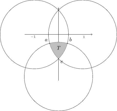
Fig. 1. Triangular domain T bounded by arcs of three circles.

Let T be a triangular domain in the complex plane C defined by

T = {z G C : |z - 6k| < V2, k = 1, 2, з} , where

6 1 = 1 , 6 2 = - 1 ,   6 3 = - i V3 .

The sets

C1 = {z G C : |z - 1| = V2} , C2 = {z G C : |z + 1| = V2^ , Сз = {z g C : |z + iV3| = V2j represent three circles in the complex plane centered at 61, 62, and 63, each of radius \/2. The triangular domain T is the common intersection of the interiors of these three circles, as illustrated in Fig. 1. The boundary of T, denoted by ∂T, consists of three circular arcs. The vertices of T are given by a = -^ (^3 - 1) (1 + i), b =2 (^3 - 1) (1 - i), c = -i, which correspond to the pairwise intersections of C1 , C2 , and C3.

2.    The Dirichlet Problem for Polyanalytic Functions

In this section, we investigate the Dirichlet boundary value problem for polyanalytic functions of order n in a bounded domain T ⊂ C. Polyanalytic functions, which are natural generalizations of analytic and harmonic functions, satisfy higher-order equations involving repeated applications of the Cauchy–Riemann operator. Our aim is to determine necessary and sufficient conditions for the solvability of the Dirichlet problem associated with such equations and to construct explicit integral representations of the solutions under suitable assumptions on the boundary data and the inhomogeneous term. We begin with the classical case n = 1 , corresponding to the inhomogeneous Cauchy-Riemann equation, and then extend the results to arbitrary order n.

Theorem 2.1 [14]. The Dirichlet problem for the homogeneous Cauchy–Riemann equation in T wz = 0 in T, w = y on dT,                           (1)

with given y € C(dT ; C), is solvable if and only if

1- [ y(Z )K 2 (z,Z ) dZ = 0 ,                              (2)

2 ni J

∂T and for z ∈ T the unique solution can be presented as

^w(z) = ^ [ Y ^{( z )K} i ^(z,Z ) d^Z, 2ni J

∂T where

Ki(z,Z) = ^-----, k=1ζ-zk and the points zk are given by

K (z,Z ) = E?---, k=5ζ-zk

Z = ^z + in,

z i = z,  Z 2 = - ¹ ,

z

- (1 + iV3)z + 1 - i \3

, z 4

(1 — i V3)z + 1 + i V3

( i y3 — 1) z — 1 — i У3 ( — 1 + i V 3) z + 1 — i ^ 3 ’

z + 1         — z + 1

z5 = =---7,   z6 = - , , z — 1         z + 1

z 7 =

— i ^ 3 z

z -

— 1

i V3

z — i ^ 3

z 8 = --^Z--- , i ^ 3 z + 1

with z 2 , z 3 , z 4 , z 5 , z 6 , z 7 , z 8 ∈ / T .

Remark 2.1. In the analytic case, the classical Cauchy integral

^{w ( z )} =

^ Z ■

2ni J Z — z ∂T already provides the solution of the Dirichlet problem. The advantage of the representation (3) with kernels (4) is that it generalizes the Cauchy kernel and remains valid in broader contexts, such as polyanalytic and k-analytic equations. While for analytic functions the two formulas coincide, the form with K1 and K2 extends naturally to higher-order equations, where the classical Cauchy formula is no longer sufficient.

Theorem 2.1 provides a complete characterization of the solvability and representation of the Dirichlet problem for the homogeneous Cauchy–Riemann equation in the domain T .

This result establishes a necessary and sufficient condition for the existence of a solution in terms of a boundary integral and presents an explicit integral formula for the solution.

Building upon this foundational result, the following theorem extends the analysis to the inhomogeneous case, where the equation involves a nonzero source term f ( z ). In this context, the solvability condition naturally incorporates both the boundary data γ and the inhomogeneity f , reflected through the integral relation involving both K i and K 2 .

Theorem 2.2. The Dirichlet problem for the inhomogeneous Cauchy–Riemann equation in T w z = f (z) in T, w = y on dT,(5)

with given boundary data y € C(dT ; C) and source term f G L 1 (T ) (in particular, f G C(T ) is admissible ) , is solvable if and only if

• 1—    [ Y(z)K2(z,Z) dz - 1 f f (z)K2(z,Z) dzdn = 0,

2ni JnJ

∂TT and for z ∈ T the unique solution can be presented as

• w(z) = 71 [ Y(z)Ki(z,Z) dz - 1 / f (z)Ki(z,C) d^dn,(7)

2ni JnJ

∂TT where Ki(z, Z) and K2(z, Z) are the kernels defined in (4).

⊳ Assume that the Dirichlet problem (1) is solvable. Then, by Theorem 2.1, the solution can be written in the form given by (3).

Let us define a new unknown function

0(z) := w(z) - T[f](z), where the operator T[f ] denotes the area integral

^{T[f](z) :}= ¹ f ^{f ( Z} )/— d^zdn-π ζ - z

T

Applying the operator d z to both sides of the definition of 0 , we obtain:

d _s 0 = d z w - d _s T [f ] .

Since w satisfies w _z = f (z) and by known properties of the area integral operator (i. e. d _z T[f ] = f ( z )), we get:

d z » = f ( z ) - f ( z ) = 0 in T.

Moreover, on the boundary ∂T , we have:

0 = w - T [f ] = Y - T [f ] on dT.

Thus, θ satisfies the homogeneous Dirichlet problem:

0 z = 0 in T, 0 = y - T[f ] on dT.                         (8)

By Theorem 2.1, the homogeneous Dirichlet problem (4) is solvable if and only if the following compatibility condition holds:

2-1 ( y (Z ) - T[f](Z))K 2 (z,Z ) dz = 0 .

∂T

We now analyze the second term using the properties of the area integral operator. The function T[f ]( Z ) is defined as:

t [f ](Z ) =

• ¹    [ f (Z ) dξ dη.

π ζ - ζ

T

Substituting this into the boundary integral, we get:

f (Z )

^Z - ^Z

d^dr) K ₂ (z, Z ) dZ

J- /T[f ](Z Mtz.C ) dZ = J- / (¹ / 2ni /                            2ni / In/

∂T                        ∂T T

= 1 [ f ( Z ) F   K²^ dZ| dldn = 1 [ f &K2M dl d)

nJ \2m — — Z             nJ

T           ∂T                        T

Therefore, the solvability condition becomes:

• 1—    I Y^(Z)K 2 ^(z,Z ) d^Z - ¹ I ^{f (Z)K} 2 ⁽z^,Z ) d^ldn = 0 , 2ni                    nJ

∂T                    T which coincides with the condition stated in (5).

Conversely, suppose that the solvability condition (5) holds. Define u(z) as in (3). Then, we can rewrite this expression in the following form:

^^(z) = Z^ I Y^(Z ) ^[K 1 ^{(z, Z} ) ^{- K} 2 ^{(z, Z )] dZ - 1} / ^{f (Z} ) ^[K 1 ^{(z, Z} ) ^{- K} 2 ^{(z, Z )] dl d}n.

2ni J                                nJ

∂T                                T

Using the result of Theorem 2.1 and the fact that the area integral tends to zero as z → ζ ∈ ∂T, we conclude that lim u(z) = y(Z), z € dT, z→ζ and clearly,

U z = f (z) in T.

Therefore, ω is a solution to the inhomogeneous Dirichlet problem (1). We now turn to the uniqueness of the solution to the problem. Suppose that U i and u ₂ are two solutions to the Dirichlet problem (1). Then, by definition, we have

(u i ) z = f in T, u i = y on dT,                           (9)

and

(u 2 ) z = f in T, u 2 = Y on dT.                         (10)

Subtracting these equations, we obtain

( u 1 — u ₂ ) _z = 0 in T, u 1 — u ₂ = 0 on dT.

This is the Dirichlet problem for the homogeneous Cauchy–Riemann equation in the domain T . By Theorem 2.1, which guarantees the uniqueness of the solution to the homogeneous problem with continuous boundary data, it follows that the only solution is the trivial one. Therefore, w1 = w2 in T, and the solution is unique. >

Theorem 2.2 establishes the solvability and integral representation of the Dirichlet problem for the inhomogeneous Cauchy-Riemann equation, which corresponds to the case n = 1 in the general theory of polyanalytic equations. The corresponding boundary condition involves a single function γ , and the unique solution is represented via the standard Cauchy-type integrals over the boundary and the domain of T , using the kernels K i and K 2 .

The next theorem generalizes this result to the case of the inhomogeneous polyanalytic equation of order n , where the unknown function w satisfies d n w = f in T , and the boundary conditions involve the traces of the first n ^-derivatives of w .

Theorem 2.3. The Dirichlet problem for the inhomogeneous polyanalytic equation in the domain T , dnw = f (z) in T, dZw = yk on dT, 0 < к С n — 1,              (11)

is uniquely solvable for f £ L 1 (T ; C) and Y _K € C(dT ; C) for 0 <  к С n — 1, if and only if for each 0 С к С n — 1 , the following compatibility condition holds:

n ¹ fi W-«          —    V-k

^   2 ni    / ^(Z ) ( a — к )! K^z, ^Z ) d^Z

+ ^{( — 1) n к} Г f (Z ) ^{(z — z) n 1} к       z ) d^dn = 0 , z £ T. (12)

n J (n — 1 — к )!

T

The solution is then given by

■*)- E (f J ^    Kz^zz ) dz

πκ к—0      дт

■    '   [        Z—z) ^{n - 1} K i (z,Z ) dd (13)

n J (n — 1)!

T where K1(z, Z) and K2(z, Z) are the kernels defined in (4).

• <1 We prove the theorem by mathematical induction on the order n £ N.

Base case: n = 1. In this case, the equation reduces to the classical inhomogeneous Cauchy–Riemann equation:

w _z = f ( z ) in T, w = Y o on dT.

The solvability condition and the integral representation of the solution are given by

Theorem 2.2. Therefore, the result holds for n = 1.

Inductive step: Suppose the theorem holds for some n = s ^ 1; that is, for the problem dZw = f (z) in T,  d^w = yk on dT, 0 С к С s — 1, the unique solvability condition and the solution formula given in the theorem are valid.

We aim to prove that the result holds for n = s + 1.

Let ω be a solution of the problem dS+1w = f (z) in T,  dZw = yk on dT, 0 < к < s.

Define the auxiliary function v(z) := dzw(z). Then v satisfies dZv(z) = f (z) in T, dZv = yk+i on dT, 0 < к С s — 1.

By the induction hypothesis, the solvability condition for v is s   /'_1W-K-1              г^-к-1

E -        (Z) l — l - 1)! K^Z) dZ а=к+1            дт       '          '

₊ ( — 1^ гf ( z )^{( Z} — zO^ - i _{K 2} (z,z ) d£dn = o

П             (k   к 1)!

T for 0 С к С s — 1. To complete the construction of w, we solve the first-order equation wz = v(z) in T, w = Yo on dT.

By Theorem 2.2, this equation is uniquely solvable if and only if

/ Y 0 ^{( Z )K} 2 ^(z,Z ) ^{dZ —} - (^v(Z)K 2 ⁽z,^Z ) ^dZdn = ⁰ -

2ni                     nJ

∂T                    T

Substituting the integral representation of v into this expression leads to the full compatibility condition for к = 0, completing the induction step.

Finally, by applying the integral representation of v and integrating once more with respect to z, we obtain the integral representation of w , matching the formula given in the theorem for n = k + 1.

Therefore, by the principle of mathematical induction, the result holds for all n G N. >

3.    The Schwarz Problem for Polyanalytic Functions

In this section, we investigate the Schwarz boundary value problem for first- and higher-order polyanalytic functions in a triangular domain T . Starting from the classical case, we derive an explicit integral representation for the solution and extend it to polyanalytic functions of arbitrary order.

Theorem 3.1 [14]. The Schwarz boundary value problem ws = f (z) in T, [Re w]+ (t) = Y(t) for t G dT,                    (14)

with given data f G L i (T ; C) , and Y G C(dT ;R) , is uniquely solvable. The solution is given by

w(z) = E ni у Y(C) (K,(z,z)— ^—^j-)dz j=1  dT C

⁺ i^{c — 1} J ^{f (Z ) K} 1 ^{( z}, ^Z ) ^dZdn ^{— 1} J ^{f (Z)K} 2 ^(z, ^Z ) ^dz dd, ⁽¹⁵⁾

T

T

where

3 2 Г c V— Im^(Z) πi j=1 ∂T∩Cj

dζ

^Z - ^e j ,

where K i (z, Z ) and K 2 (z, Z ) are the kernels defined in (4) .

The solution w ( z ) in (14) can be expressed more compactly as

^^(z) = S [y ] ^{( z )} + T [ f ] ^{( z )} + ic,

where the operators S [ 7 ] and T[f ] are given by

SM(z) = Eni / 7(Z) (Ki(z,Z) _      ) de, j=1 ∂T∩Cj

T [f ](z) = - 1 1 f (Z )K i (z,Z ) d^dn - 1 1 f (Z )K 2 (z,Z ) dd

T

T

We now introduce the poly-Schwarz operator S _n in the domain T , defined for data 7 o ,7 i , - - .,7 n - i E C (dT ; R), as

n __1 (_i)k ³ 1 г             ______

Sn [7o ,71>---,7п-1](2) = Е-П-£- / (Z _ z + Z _ z)k 7k(Z) k! ni

^{k =0        j =1}    ∂T ∩ C j

X KK-zz,) ) ^_

} dZ- (20)

^{Z - e}j /

It is clear that for n = 1, this operator reduces to the classical Schwarz operator: S o [ 7 ] = S [ 7 ].

• 3.1.    Boundary properties of the Poly-Schwarz operator. We investigate how the poly-Schwarz operator behaves near the boundary of the domain. The results confirm that it reproduces the given real-valued boundary data for all relevant derivatives.

Theorem 3.2. If7 0 ,7 1 ,...,7 _n- i E C(dT ;R) , then

∂n dzn Sn[7o,71,---,7n-i](z) = °, z E T-

⊳ By the definition of the operator S _n in (15), we have

S n [ 7 0 ,7 1 , - - - ^,7 n - i ^{]( z )}

K i (z,Z ) _ z~_:^~) dZ

= E (# 17 Ji / [«- z +- Г 7k к ^{k =0        j =1} ∂T ∩ C j

= E (# E 0 ( _ i)k ^{_ l} (z+E ^ / К+оч (z ) (K^z) _ ^У k =0         l =0                          j =1    _{∂T∩C j}                                   ^j

Now define

7 k,i ^(Z ) ^{:    (Z} + ^{Z )} l 7 k ^(Z ) >

and set

S [ Y k,i ]( z ) := E • / Y k,i ( z ) f K i ( z,z )    .     ) dC                (21) πi                           ζ - ǫ j j = i    dT H C j

Thus, we obtain:

n — 1

Sn[Y0, • •• ,Yn—i](z) = £ k=0

TTE C yDk'^-l ( z + *- l S ^W- l =0

Each term S [ Y k,l ]( z ) is independent of z, since it is defined via integration over the boundary with kernels K i (z,Z ) and Y k,l (Z )• Therefore, all z-dependence is inside the polynomial ( z + z ) ^{k —} l .

Differentiating n -times with respect to Z, we obtain:

But for all k — l < n , the n -th derivative of the polynomial (z + z) ^{k — 1} vanishes. Since k ^ n — 1, we always have k — l < n , so each term is zero.

Hence,

∂n dzn Sn[Y0, • • • ,Yn—i](z) = o. [>

Having established the vanishing of the n -th z -derivative in the domain, we now describe how the lower-order derivatives of the poly-Schwarz operator behave on the boundary.

Theorem 3.3. If y o , Y i , • • •, Y n - 1 € C(dT ; R) , then

| Re [ d_ S n [y o , Y i , • • •, Y n — i ]( z )]} ( t ) = Y i (t), t € dT, l = 0,...,n — 1 ,       (22)

where the operator S _n is defined by equation (15) .

<1 We prove the identity for each l = 0,1, • • •, n — 1. For l = 0, we simply have dzo Sn[Y0,Yi, • • • ,Yn—i](z) = Sn[Y0,Yi, • • • ,Yn—1](z)•

According to Theorem 3.1, the non-tangential boundary value of its real part satisfies n—i

{ Re[Sn[Yo,Y1,•••,Yn—i](z)] }+(t) = E k=0

EE k!

E (k) l =0

^{( —} t ^— ty l ^Y ki ^(t),

where the functions γ _k,l are defined as in equation (17).

Note that for k ^ 1, the term ( — t — ^z + t + t) ^{k —}l = 0. Hence, all terms vanish except the one with k = 0, giving

{ Re[ S n [ Y o ,•••,Y n — i ]( z )] } ⁺ ( t ) = Y o ( t )

Thus, equation (19) holds for l = 0.

Now, let l = 1,2,...,n — 1. Differentiating under the integral sign (justified by the continuity of γk), we obtain dl                            n^ (—1)k-l 3, i

—Sn [Yo,...,Yn-i](z) = ^-77—niE-dz1                             (k — l)! ^^ ni k=l          j=1

X I ( Z — z + Z — z )^k - Y k ( Z ) (ki(z,Z ) — ∂T ∩ C j

^Z - ^e j

dζ.

Expanding the power term and reorganizing, we get

E E f - 0 < — ( z + zWm S МД z G T.

k=l ⁽ k   ^{l )!} m =0    m /

Taking the real part and applying the non-tangential boundary limit, we obtain l                            + n-1      k-l k-l

|Re dLS „ [ Y o ,..., y.-i]_W    ( t ) = E ^ E (km 0 ( — t — tY - l - m Y kU t ) .

k = l         m =0

Again, only the term with k = l and m = 0 survives since all other terms involve powers of zero. Hence,

{Re fdLSn[7o,...,7n-1](z)j } (t) = yiott) = Yi(t), which proves equation (19) for all l = 0,..., n — 1. >

• 3.2.    Pompeiu operator on the triangle. In this section, we introduce the following area integral defined by

T i [ f ]( z^^ — 7m ff( Z — z + Z — z ) ^{l -} 1 [ f ( Z ) K i ( z,Z )+ f ( Z ) K 2 ( z,Z )1 d^n,     _z ,

^{n ( l — 1)!} T                                                                    (23)

z G T, l = 1, 2,..., for functions f G Li(T; C).

The operator T _l is referred to as the Pompeiu-type operator in this context. In particular, for l = 1, it reduces to

Ti[f ](z) = T[f](z), z G T.

We also define

To[f](z):= f (z), z G T, and this operator satisfies the following relation:

∂

—T[f](z)= To[f ](z), z G T.

This operator family satisfies a recursive relation involving complex conjugate differentiation. The following theorem establishes this fundamental property.

Theorem 3.4. If f G L i ( T ; C) , then

∂

—T i [ f ]( z )= T i - i [ f ]( z ) ,   z G T, l = 1 , 2 ,...,n — 1 .

<1 Let f G L i ( T ; C ), and let us consider the operator

T i [f ](z) = _П^)! U' ( Z - z + —) l ^{- 1} [ f ( Z ) K i ( z, z ) + f (Z )K 2 (z,Z )] d^ dn.

Note that z — z + z — z = (z + z) — (z + z) = 2 Re(z — z), which is a real-valued function depending smoothly on z . Define

^( Z,z ) := (Z — z + Z — z ) l ^- 1 .

Differentiating under the integral sign with respect to z , we obtain

^Tff » = 4Дм I^«,z )] [ f (Z)K i (z,Z ) + f (Z)K 2 (z,Z )] d^dn-∂z            ⁿ(l - ¹ ) ^! -T ^dz

Now observe that

—Ф( Z, z ) =     Z - z + Z - z =    (2 Re( Z - z )) ^{l -} 1

∂z         ∂z                   ∂z

= dz ( ^z +^z - z - z ) l ¹ = ^-(l - ¹⁾ ( ^z - z + ^z - z ) l ² .

Thus, dTi[f](z) = П-Л)(-(l - 1)) Л(Z - z + Z-z)l-2 [f(Z)Ki(z,Z) + f(Z)K2(z,Z)] dzdn-

Simplifying the constants, we get dTi[f](z) = П--?1! Л (Z - z + Z-z)l-2 [f (Z)Ki(z,Z) + f (Z)K2(z,Z)] dzdn-

This is exactly the definition of T i - i [f](z). Therefore, we conclude that

—T i [f ]( z )= T i - i [f ]( z ) ,    z G T. [>

Theorem 3.5. Let f G L i ( T ; C ) . Then, for each l = 1 , 2 , 3 ,... , the real part of the Pompeiu-type operator T i [f ] satisfies

{Re Ti [f]}+ (t) = 0, t G dT, where {·}+ denotes the nontangential boundary limit from within the domain T .

⊳ Let z ∈ T and consider

T i [f ]( z ) = П ^ -ля Л (Z - z + Z-^ ) ^{l - i} [ f ( Z ) K i ( z,Z ) + f (Z)K 2 (z,Z )] d&n

Note that _

Z - z + Z - z = (Z + Z) - (z + z) = 2 Re(Z - z), so the kernel is real-valued:

(Z - z + 7—zz ) ^{l - 1} € R .

Then,

^Re Tf ^{]С г )} = П —Л)! U ⁽² Re⁽ Z — z^ - R^e f ( Z ) K i ( z, Z ) + fZK&Z) ] d^ dn

As z ^ t € dT nontangentially, the kernel (2Re(Z — z))l-1 becomes symmetric with respect to the reflection across the line Re(Z) = Re(t). Due to this symmetry and the regularity of the data f ∈ Lp , we have lim Re Ti [f ](z) = 0.

z → t ∈ ∂T      ^l

Hence,

{ Re Tf ] } ⁺ ( t )=0 , t € dT. [>

We now consider the Schwarz-type boundary value problem for the inhomogeneous poly-analytic equation in the triangular domain.

Theorem 3.6. The Schwarz-type boundary value problem for the polyanalytic equation dzn^(z) = f (z),   z € T, f € L1(T; C),                         (28)

subject to the boundary conditions

{ Re (d» } ⁺ ( t ) = Y s ( t ) , t € dT, Y s € C(dT ; R) , s = 0 ,..., n — 1 ,          (29)

and the integral normalization conditions

^ — / I^m(d>^{( z} )) d^Z = c _s ,  s = ^{0 ,} ...^,n - ¹ ,

πi            z ζ - ǫj j"1   dTHCj is uniquely solvable. The solution is given by

- 1 (z + z) ^s

^(z) = Sn[Y0,Yi, • • • ,Yn-i](z) + Tn[f](z) + £----p-iCs, s=0 s’ where the operators Sn and Tn are defined in equations (15) and (21), respectively, and cs ∈ R are given constants for s = 0,... ,n — 1.

⊳ We aim to solve the boundary value problem dMz)= f (z), z € T, subject to the boundary conditions

{Re(dfw)}+ (t) = Ys(t), t € dT, s = 0,...,n — 1, and the normalization conditions

^ — / Im (ds^(z)) dZ = cs, s = 0,...,n — 1. πi            z      ζ - ǫj j"1   dTHCj

We construct the solution as follows:

n — 1

(z + z)s .

ic s . s !

w(z) = Sn[YO,Y1, • •- ,Yn—1](z) + Tnf](z) + £ s=0

Let us denote:

V¹ (z + z) s

W 1 (z) := S n [ Y o ,---,Y n — 1 ]( z ) , ^ 2 ( z ) := T _n [f](z),   W 3 ( z ) := V  --- i-s-ic_s.

s !

s =0

We will verify that w = W 1 + W 2 + W 3 satisfies the differential equation and both boundary conditions.

Step 1: Verify the differential equation. By definition of the operator Tn[f ], we have dZTn[f](z)= f (z),  z G T.

Also, since S _n is constructed from boundary data, it is a solution of the homogeneous equation:

d n S n [ Y o , - - -, Y n — i ]( z ) = 0 , z G T.

Likewise, W3(z) is a polynomial in z + z, and hence satisfies dnw3(z) = 0, z G T-

Therefore,

& n w(z)= f ( z ) , z G T-

Step 2: Verify the real part boundary conditions. From the construction of S n [ Y o , - - -, Y n — 1 ], we have

{ Re( d s S n [ Y o , - - -, Y n — 1 ]) } ⁺ ( t ) = Y s ( t ) , t G dT-

On the other hand, it was previously shown (see Pompeiu operator properties) that

{ Re(d s T n [f](z)) } ⁺ ( t ) = 0 , t G dT, s = 0,---,n - 1 -

And since W 3 is a real polynomial multiplied by i, its real part vanishes:

Re ( d s w ₃ ( z )) = 0 -

Hence,

{ Re ( d s w ) } ⁺ ( t ) = Y s ( t ) , t G dT-

Step 3: Verify the normalization conditions. We compute:

d f w ( z ) = d f w ₁ ( z ) + d f w ₂ ( z ) + d f w ₃ ( z ) , s = 0 , - - -, n — 1 -

By construction, the imaginary part of d s W 1 and W 2 satisfy

^ — / Im ^{( d} s ^w 1 + ^2)     = 0 -

πi             z z ζ - ǫj j = 1 dTC

Meanwhile, the contribution from W 3 is

( \     (z + z)s • d^3(z) = —s— ics, so

s

Im(d>3(Z)) = (^^ cs, and using Cauchy’s theorem and symmetry, it can be shown that the integral condition gives

^2 - I Im(d!«3(()) -d- = cs. πi            z ζ - ǫj j-1   dTHCj

Thus, the full normalization condition is satisfied. ⊲

Acknowledgments. The author is very grateful to the referees for their valuable suggestions, which have helped improve the quality of this paper.