Classification of Dynamical Systems Near a Cosymmetric Equilibrium

1.    Problem Statement

The theory of cosymmetry was founded by V. I. Yudovich [3] to explain an unusual effect in the problem of plane filtration convection posed by D. V. Lyubimov [4]. According to his definition, a mapping L : H x Л ^ H in the Euclidean space H = R ⁿ , Л C R ^m is called a co-

• ^# The work of L. G. Kurakin was carried out as part of Topic no. FMWZ-2022-0001 of the State Assignment at the Institute of Applied Physics, Russian Academy of Sciences (Registration no. 122041100222-7). The work of A. V. Kurdoglyan was performed at the North Caucasus Center for Mathematical Research, VSC RAS, with support from the Ministry of Science and Higher Education of Russia (Agreement no. 075-02-2025-1633).

• (c) 2025 Kurakin, L. G. and Kurdoglyan, A. V.

symmetry of a mapping F : H x Л ^ H, or of the differential equation ui = F(u,A), u g H, A G Л,

if F and L are orthogonal at every point u G H for any fixed value of the parameter A G Л .

Let u = u o G H be an equilibrium of system (1) at A = A o G Л . This equilibrium is called cosymmetric if it is also a zero of the cosymmetry:

^F(u o , ^A o ) = ^L(u o , ^A o ) = °.

In what follows, we assume that the mappings F and L are analytic. If given equilibrium of the system is non-cosymmetric with respect to a specified cosymmetry, then, in the absence of additional degeneracies, it belongs to an analytic family of equilibria. As later shown by L. G. Kurakin [5], the converse also holds. In the neighborhood of a cosymmetric equilibrium, V. I. Yudovich studied the properties of cosymmetry in a sufficiently general form for applications to the filtration convection problem. In particular, for a system with a real parameter, the cosymmetry was assumed to be a linear skew -symmetric operator L* = —L independent of the parameter. For an odd-dimensional system, such an operator is non-invertible. By replacing the skew-symmetry of a linear cosymmetry with the less degenerate requirement of its local invertibility, and by allowing the cosymmetry to be a nonlinear operator depending on a real parameter, we are led to the problem of analyzing the bifurcations of the system in a neighborhood of a cosymmetric equilibrium.

This study was carried out in [6] using the Lyapunov–Schmidt method [7], where it was shown that the dimension of the kernel of the linearization at a cosymmetric equilibrium has the same parity as the dimension n of the original system. Moreover, in an odd-dimensional system with one-dimensional kernel, the cosymmetric equilibrium belongs to an analytic family of equilibria. Consequently, according to the results of [5], the original system also admits another cosymmetry for which this equilibrium is non-cosymmetric. Bifurcations in evendimensional systems with a two-dimensional kernel were described. Thus, the problem arises of a more detailed study of system (1) by means of the center manifold method [8] under the following assumptions:

• 1 ° . n is even.

• 2 ° . The point u o is an equilibrium of system (1) for all A :

F (u o ,A) = 0 V A G Л.

• 3 ° . The equilibrium u o is cosymmetric for all A :

L(u o ,A)=O V A G Л.

• 4 ° . The cosymmetry L(u, A) is invertible in a neighborhood of the point u = u o for all A G Л .

• 5 ° . The Jacobian of F at (u o , 0) has a two-dimensional kernel:

F 9 V    ^dF(u, ⁰⁾

.

u = u 0

dimker Fo = 2,    Fo := ------- du

• 6 ° . The entire stability spectrum of the matrix F o , except for the double zero eigenvalue, lies strictly in the left half-plane.

Under assumptions 1 ° - 6 ° , the center-manifold reduction of system (1) yields the following two-dimensional system of differential equations in the Euclidean space:

x = f ^(x,y^,A')’ y = g(x,y,X)                              (2)

with variables (x,y) G Q C R ² and m -dimensional ( m ^ 1 ) parameter A G Л C R m , defined in a small neighborhood of the point 0 G V := Q x Л .

Remark 1. In this paper, the theory of the center manifold is invoked only insofar as it allows the reduction of the original higher-dimensional system (1) to the two-dimensional system (2). Moreover, one may instead begin with the two-dimensional system (2) and develop the classification for it, reducing the higher-dimensional case to the two-dimensional one by means of the center manifold theory under assumptions 1 ^° - 6 ^° .

Let the mapping

L° : V H R2 : (x, y,A) H f L1(x’ y’ A) ) ,y’ ’ V L2(x,y,X) J denote the cosymmetry of system (2) inherited from system (1) via the center-manifold reduction:

f(x,y,A)L i (x,y,A) + g(x,y,A)L 2 (x,y,A)=0, (x,y,A) G V.               (3)

We further assume that system (2) satisfies the following properties:

• 1 ° . The mappings f , g , L i , and L 2 are analytic in the neighborhood V .

• 2 ^й . System (2) has the zero equilibrium for all A G Л , so that the functions f and g : V H R satisfy the condition

f (0,0,A)= g(0,0’A)=0,  A G Л.                           (4)

• 3 ° . The equilibrium x = y = 0 is cosymmetric for all A G Л , so that the equality

L ^° (0, 0, A) = 0,   A G Л,

is satisfied.

• 4 ° . The cosymmetry L ° is locally invertible in a neighborhood of the point x = y = 0

  at A = 0 :

  
  

  det B = 0,

  
  
  
  

  dL i (x,y,0) ∂x dL 2 (x,y,0) ∂x

  
  

  dL i ( x,y, 0) ∂y dL 2 ( x,y, 0) ∂y

  
  

  x = y =0

  
  
  
  

5 ° . The linearization matrix A of system (2), (4) at the zero equilibrium for A = 0 has the two-dimensional kernel:

dimker A = 2,

A :=

/ df ( x,y, 0) ∂x

I dg ( x,y, 0)

∂x

df ( x,y, 0) ∂y dg ( x,y, 0) ∂y

)

= 0.

x=y=0

Remark 2. Properties 2 ° - 5 ° are inherited by system (2) from system (1). Property 1 ° , however, need not be inherited. Indeed, even if the mappings in the original system are analytic, the center manifold may fail to be analytic. For the results obtained below, the analyticity assumption on the subsequent mappings, as well as on the functions f , g , L i , and L 2 , is adopted merely for convenience and is not essential. Throughout the paper, analyticity may be replaced by C ⁴ -regularity.

2.    Effect of Cosymmetry on the System’s Structure

The following theorem states.

Theorem 1. Under assumptions 1°-5°, system (2) can be written in the form x = -L2(x,y,X) h(x,y,X), y = Li(x,y,X) h(x,y,X),                (8)

where the function h : V ^ R is analytic in the neighborhood V and satisfies

h(0, 0, 0)=0.                                       (9)

⊳ According to the inverse function theorem, conditions (5) and (6) imply that the system of equations

K1 = Li(x,y,X),  K2 = L2(x,y,X), has a unique solution x = X (Ki,K2,X), y = Y (Ki,K2,X), which is analytic in the variables K1 , K2 and in the parameter λ in a small neighborhood of the origin. Substituting this solution into the identity (3) and viewing it as an identity in the variables K1 and K2 , we obtain

K i f i (K i ,K 2 , X) + K 2 g i (K i ,K 2 , X) = 0,                       (10)

where f 1 and g 1 are analytic functions of K 1 , K 2 and the parameter λ in a neighborhood of the origin:

fi(Ki,K2,X) := f (X(K1,K2,X), Y(Ki,K2,X), X), gi(Ki,K2, X) := g (X(KiK X), Y(KiK X), X) .

It follows that f i (K i , 0, X) = g i (0, K 2 , X) = 0 for all sufficiently small values of K i , K 2 , and X .

Hence, the functions f1 and g1 can be written in the form gi(Ki,K2, X) = Kihi(Ki,K2, X), fi(Ki,K2, X) = -K2h2(Ki,K2, X), where h1 and h2 are analytic functions of K1 , K2, and the parameter λ in a neighborhood of the origin. It follows from the identity (10) that hi = h2.

Thus, equations (2) can be rewritten in the form (8), where the function h is defined by

h ( x, y, X ) := h i ( L i ( x, y, X ) , L 2 ( x, y, X ) , X )

and is analytic in the neighborhood V .

Now let us prove that h(0, 0, 0) = 0 . It follows from (2) and (8) that

g ( x, y, X )

^h(x,y^,X) = —₍----- tv.

L i ( x, y, X )

By the analyticity of the functions g and L i , from condition (4) and assumptions 4 ° and 2 ° we obtain the following asymptotic expansions for small x , y и λ :

L i (x, У, X) = l i x + l 2 y + O(x ² + y ² + ( | x | + | y | ) • | X | ) , g^(x,y, ^X) = Ox ² + y ² +^{( | x |} + Ы) • ^{| X |} ) .

It follows from the condition det B = 0 that 1 2 + 1 2 =0 . Taking the limit, we obtain the equality (9):

h(0,0,0) = lim ^x^

^v , , ^J    x ^ o L i (x, 0, 0)

h(0, 0, 0) = lim ^{g (0 ,}y, ⁰⁾ _: ^{V 7}   y^ o L i (0,y, 0)

O(x ² )

= lim x >0 lix + O(x2)

= 0   (l i =0),

O(y ² )

= lim / ox y^ o 1 2 У + O(y ² )

= 0 (I 2 = 0). >

Theorem 1 reduces the problem of studying the properties of the original system (2), (4) under assumptions 1 ^й - 5 ^й to system (8), in which the functions L i , L 2 , and h are analytic in the neighborhood V and satisfy the conditions (5), (6), and (9).

The phase portrait of the system (8) for each fixed value of λ can be constructed by combining the phase portrait of the equations x = —Li(x,y,A), y = Li(x,y,A)

with the set of equilibria S of the system (8):

S := {x, y E Q : h(x, y, A) = 0 } .

The system (8) always possesses the cosymmetric zero equilibrium. Each of its nonzero equilibria is noncosymmetric, lies on some phase trajectory of the system (11), and separates it into two parts, which are trajectories of the system (8). In the region where h(x,y,A) <  0 , the directions of motion along the phase trajectories of the systems (8) and (11) are opposite.

3.    Stability of Equilibria The linearization matrix of the system (8) family (12) has the form at an equilibrium (x, y) = (а, в) of the A (а, в, A) -Li^.A) «g^ Li(a,e,A) 2^^ -Li^.A)   a Li(a,e,A) У=в У=в

The eigenvalues of the matrix A (а, в, A) are zero, and its trace is given by

N := tr A (а, в, A).

In particular, A (0, 0, A) = 0 , so that dimker A (0, 0,A) = 2 .

Consider the equilibria (12) with x ² + y ² = 0 . If N = 0 , then dimker A (а, в, A) = 1 , and, according to the cosymmetric version of the implicit function theorem [3], each nonzero equilibrium of the family (12) is nonisolated and belongs to the one-parameter family of equilibria. The equilibria of (12) with N > 0 are unstable. When N < 0 , the stability problem for the equilibria of the family (12) of the system (8) corresponds to the critical case of a simple zero eigenvalue. This case was studied by Lyapunov A. M. (see [9], Theorem of Section 32, degenerate case). According to his results, the equilibria of the family (12) with N <  0 are the Lyapunov stable and asymptotically stable in the directions transverse to the family S . In the present work, for N = 0 , a situation arises where the linearization matrix A (а, в, A) has a double zero eigenvalue, while dimker A (а, в, A) = 1 . In this case, the equilibrium (а, в) , called a boundary equilibrium [6], is non-isolated, and its stability problem requires a nonlinear analysis. This boundary equilibrium locally separates the family S into two arcs, each of which consists entirely of either linearly stable or linearly unstable equilibria.

4.    Model Systems and the Principle of Their Classification

In addition to assumptions 1й- 5й, let the following condition hold for the system (8): 6й. The inequality hio + h0i = 0,

is satisfied, where hio := ^xy^I x=y=

Without loss of generality, assume that

1, dh(x,y,o) I , h ^{oi :}= dy |

.

h oi = 0.

The case h io = 0 can be reduced to this one by interchanging x О y and f о g . Let E o := h(0, 0, Л) . The change of variables

x ^ x, y ^ h(x, y, Л) - E o

in the system (8) brings the function h to the form E o +y , thereby straightening the family (12).

Expanding the right-hand side of the resulting system in the Taylor series in the variables x and y , we write it in the asymptotic form as | x | + | y | + | Л | ^ 0 :

^x = [Mx.y,^ + Of ^(x,y.^)] • ^(E o + y), ^y = [ g o ^(x, y, ^) + ^O(g^(x, y. ^Л)) ] • ^(E o + y).

where

fo(x. y, ^) := (aio + №) x + 0)1 y, go(x, y, ^) := (aio + ^i) x + (aoi + де) y + (a2o + ^2) x2 + a3o x3,

and

^f(x,У^{,Л) :}= ^x 2 + y ² + | y | •^{| Л |} + ^{| x |} •^{| Л | 2} , g(x,y^) := | x | ⁴ + | xy | + y ² + ( | x | ³ + | y | ) • | Л | + | x | • | Л | ² .

The quantities a io , a oi , a io , a oi , a 2o , a 3o are real coefficients of the system (18). Let ^ := ( e o , ^ o ,^ i ,^ 2 ,^ 3 ) denote a new small parameter whose components are functions of the m -dimensional parameter λ . We assume that the five components of µ are independent. This situation occurs in the generic case when m ^ 5 .

Neglecting in (18) the terms insignificant for further consideration, we obtain the system:

x = f o (x. y, m ) • ( e o + y). У = g o (x,y,^ • (E o + y).

Its cosymmetry

L (x.y.o)^' gf'y^n

-f o (x,y,v)

is invertible and vanishes at the equilibrium x = y = 0 . Thus, system (20) with cosymmetry L satisfies assumptions 1 ° - 6 ° .

Note that the symmetry between the variables x and y in system (20) is broken due to condition (16) and the transformation (17).

The further analysis of equations (8) reduces to the study of system (20), whose coefficients and small parameters can be regarded as arbitrary, provided that they satisfy the inequality det B = a io a oi — a oi a io = 0, where the matrix B , according to definition (6), has the form

B=

a 10

^{— a} io

a 01

^{— a} oi

.

The system corresponding to equations (11) takes the form:

^x = ^f o ^(x,y^,^⁾. ^y = g o ^(x,y.^⁾-

The linearization matrix

M :=

∂f 0 (x,y,0) ∂x

∂g 0 (x,y,0) ∂x

∂f 0 (x,y,0) ∂y

∂g 0 (x,y,0) ∂y

^a 10

^a 10

^^^"

^a 01

^a 01

)

of the system (21) at the zero equilibrium for ^ = 0 is invertible, since det M = det B = 0. The classification of the zero equilibrium of system (21) in generic case det M = 0, trM = 0,  dM :=tr2M - 4det M = 0

is as follows:

Node:   det M> 0, dM > 0;

Focus:  det M > 0, dM < 0;

Saddle: det M < 0.

The invariants (23) are expressed by the formulas:

det M = a1oao1 — ao1a1o,  trM = a1o + ao1, dM = («10 — aoi)2 + 4«oi aio.

The linearization matrix of the system (20) along the family of equilibria y = —Eo has the form

( 0 f o (x, — E o ,^) \ 0 g o (x, — E o ,^)

Setting the eigenvalue g o (x, — E o ,^) equal to zero, we obtain the cubic equation

(a io + ^ 1 ) x + (a 2o + №) x ² + a 3o x ³ = (a oi + ^ o ) E o ,

which determines the boundary equilibria (x, — E o ) of the family y = — E o . These equilibria separate the family y = — E o into several connected sets of the type interval or ray, within each of which the equilibria are either linearly stable or unstable. If the multiplicity of at least one of these roots is greater than one, then when passing from the system (20) to equations (18), the number of boundary equilibria may, in general, change. In the generic case, all real roots of the polynomial (27) are simple. The number of such real roots is determined solely by the nondegeneracy conditions.

We construct a classification of the system (20) according to the following set of properties, which are preserved under the perturbation of the system (20) to (18):

• 1 * Type of the cosymmetric equilibrium of (11): node / focus / saddle.

• 2 * Number of boundary equilibria of the family y = — E o of (8): 0 / 1 / 2 / 3 .

• 3 * Relative position of the cosymmetric equilibrium x = y = 0 and the family y = — E o . The family y = — E o lies in the lower half-plane, on the x -axis, or in the upper half-plane: sgn E o = 1 \ 0 \ — 1 .

• 4 ^* Vector of separatrix intersections (only for a saddle equilibrium):

v := (v i , V 2 , V 3 , V 4 ),                                            (28)

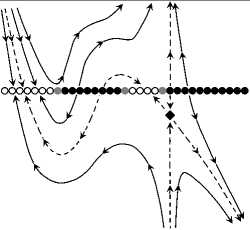
where the j-th component denotes the number of intersections of the j-th separatrix of the saddle of the system (21) with the equilibrium family y = —Eo . The separatrices are numbered counterclockwise around a sufficiently small circle centered at the origin, starting from the vector (x,y) = (0,1) (inclusive).

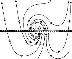
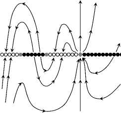
For example, v = (0,1,1, 0) in Fig. 1 (c 1 ) , and v = (0, 0, 0, 0) in Fig. 1 (c ₀ ) .

In the sequel we impose nondegeneracy conditions on the coefficients of (20) on which properties 1 * and 2 * depend. These properties also depend on certain small parameters of (20). Setting the remaining coefficients and small parameters to zero yields a truncated system . By further simplifying the truncated system via invertible changes of variables and time rescaling we obtain a model system . Considering each model system under all nondegenerate relations among its small parameters, we classify the model systems according to properties 1 * - 4 * . Degenerate parameter relations, i. e. relations for which at least one of the properties 1 * - 4 * of the model system ceases to persist under the passage first to the system (20) and then to its perturbation (18), are omitted. Moreover, two systems are regarded as belonging to the same class if they coincide up to an invertible analytic change of variables x , y , a time reparametrization t ( including time reversal ) , and a reparametrization of µ .

Table 7 lists all truncated and model systems considered in this work.

Class names are formed as follows:

• 1)    Choose the letter (a)– (h) of the model system (see Table 7) to which the class belongs.

• 2)    Append indices corresponding to the discriminating signs of certain functions of the parameter ^ . Instead of the usual sign function sgn x we use the function w defined by

  1,

  
  

  w(x) := 0,

  
  

  x >  0,

  x = 0,

  
  
  
  

_2, x< 0,

• 3)    If the equilibrium x = y = 0 is a saddle, append indices corresponding to the separatrix intersection vector v to the model system letter (a)–(h).

5. Classification of the System (20) by the Codimension of Degeneracy

Generic Case. Assume that a io = 0 . The truncated system derived from equations (20) has the form:

x = ( a io x + a oi y) • (e o + y), y = (a io x + a oi y) • (e o + y).

The change of variables x ^ aiox + aoiy, y ^ У| det M| • y, reduces it to the model system x = (aix - siy) • (ei + y), y = x • (£1 + y), ai = 0, si = ±1, where trM                ,                 eo ai := —^^^^=, si := sgn det M, Ei := —^^^^=.

71 det M |                           71 det M |

Remark 3. The system (32) retains its form under the transformation x ^ — x , y ^ — y , t ^ — t , E i ^ — Ei. Therefore, without loss of generality, we may assume that E i ^ 0 .

The classification of system (32) is presented in Table 1 and the corresponding Fig. 1.

Table 1

Classification of system (32) in a neighborhood of the equilibrium x = y = 0

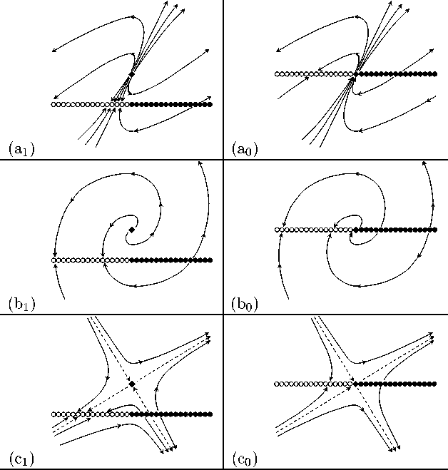
Fig. 1. Phase portraits of the model system (32) corresponding to the classification in Table 1. Here: О \ О — cosymmetric \ non-cosymmetric equilibrium;

O\® \^ — stable \ boundary \ unstable equilibrium; dashed lines are separatrices of the saddle equilibrium of system (32).

Class	Conditions
	s i , a i	sgn S i
(a i )	s i = 1, a i >  4	1
(a o )	( node )	0
(b i )	s i = 1, a i <  4	1
(b o )	( focus )	0
(c i )	S i = — 1	1
(c o )	( saddle )	0

Case of a Single Degeneracy. Let a10 — °, a20a01 — 0,   aio — a01-                           (34)

The system truncated from equations (20) and given by x— awx • (eo + y), y — (mx + aoiy + a20X2) • (eo + y),              (35)

is transformed, by a change of variables and, when a2o < 0, a reversal of time, x ^ VKol x, y ^ aoi sgna2o • y, t ^ sgna2o • t,

to the model system x = a2X • (£2 + y),   y= (vix + y + x2) • (e2 + у),   a2 = °, 1-

The coefficient and parameters of the model system (37) are given by

• a io           sgn a 20

a2 :=---,   vi :=    ---- • ^1, £2 := aoi sgn a2o • £o-

• a oi            Vl a 2o l

Let us denote by

6i(a,b):= a2 - 4b(39)

the discriminant of the polynomial x ² + ax + b .

Remark 4. The substitution x ^ —x in (37) changes only the parameter v i and the intersection vector:

v i ^— v i , v ^ (v i , V 4 , V 3 , V 2 ).

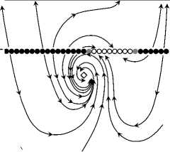
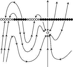
The analytical classification of the system (37) is summarized in Tables 2 and 3, and the corresponding phase portraits are shown in Fig. 3.

Theorem 2. In the classification of (37) , all classes not appearing in Tables 2 and 3 are empty:

^(d i2 ),  ^(d o2 ),  (© ii ),  ^(e i2 ),  ^(e i2 ), ^(e 2i ),  ⁽e o2 ),  ⁽e 22 ),  ^(e 22 )-                      ⁽⁴⁰⁾

Table 2

Classification of the system (37) in a neighborhood of the node x = y = 0 in the space of small parameters v 1 and £ 2 . Here 5 11 = v ² + 4£ ₂ . The classes are written in the form (d _w(_{E 2} ),_w(j ₁₁ )), where the function w is defined by (29)

Class	Conditions			Example (a = 0)
	a 2	sgn £ 2	sgn 5 ii	ε 2	ν 1
(d ii )	a 2 >  0	1	1	α 2	α
(d 21 )	a 2 = 1	- 1		- a 2	3a
(d 01 )	( node )	0		0	α
(d 22 )		- 1	- 1	- a 2	α

Table 3

Classification of the system (37) in a neighborhood of the saddle x = y = 0 in the space of small parameters v 1 and £ 2 . Here 5 11 = v ² + 4£ ₂ , 51 2 = 77-2^2 v2 + 4 e₂ . The classes are written in the form fe ^w(i 12 )     Л

• ¹²      (1 - a ₂ ) ^{2 1        2 .}                                                            w(ε 2 ),w(δ 11 ) ^,

where the function w is defined by (29)

Class	a 2	Conditions		Sgn 5 12	Example (a = 0)
		Sgn £ 2	sgn 5 ii		ε 2	ν 1
(e 1i )		1			α 2	α
(e 2i )	a 2 < 0	- 1	1	1	— (1 — 2a 2 ) a 2	3(1 - a 2 )a
(e 0i )	( saddle )	0			0	α
(e 2i )		- 1	1	- 1	2 (a 2 - 2 (1 - a 2 ) 2 ) a 2	4 (1 - a 2 )a
(e 22 )		- 1	- 1	- 1	- a 2	α

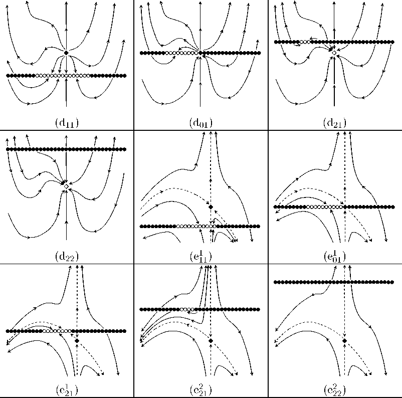
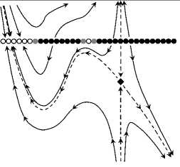
Fig. 2. Phase portraits of the model system (37) corresponding to the classification in Tables 2 and 3.

First Case of Double Degeneracy. Let aio = 0, аю = aoi, a2oaoiaoi = 0.

The system, truncated from equations (20), is given by x = ((aoi + Цз) x + aoiy) • (eo + y),   y = (mx + (aoi + Vo) y + a2ox2) • (eo + y),(42)

and can be reduced to the form x = (x + V2X + y) • (ез + y), y = (V3X + y + x2) • (ез + y),(43)

by a change of variables and of time, and by time reversal, when a 2o < 0 :

a 2o a oi x ^            ^ x’ (a oi + V o ) 2	2 a 20 a	(a oi + V o ) 4 , t ^                • t' a 20 a 2 01	(44)
	у ^            • y, (a oi + Vo)
The parameters ν 2 , ν 3 , and ε 3 are	determined by
V 3 - V o	_ ,      aoi V i	2 _ ,    a2o a oi E o
v 2 •=       ,     ’ a oi + V o	(a oi + V o ) 2	°     (a oi + V o ) 3	(45)

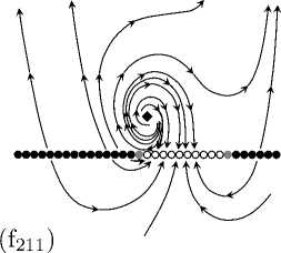
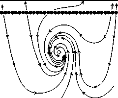
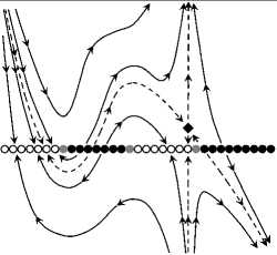
The classification of the system (43) is presented in Table 4 and illustrated in Fig. 3.

Table 4

Classification of the system (43) in a neighborhood of the equilibrium x = y = 0 in the space of small parameters v ₂ , v ₃ , and e ₃ . Here S 13 = v 2 + 4v ₃ , S 14 = v 2 + 4e ₃ . The classes are written in the form (f _w(j ₁₃ ),_w(i ₁₄ ),_w(_E 3)) , where the function w is defined by (29)

(^f 210 )

^(f 2i2 )

^(f 222 )

Fig. 3. Phase portraits of the model system (43) corresponding to the classification in Table 4. The case where the zero equilibrium is a focus (v 2 + 4v ₃ < 0).

Second case of double degeneracy. Let

• a10 — a20 — °, a30 aoi — 0,   Gio — a01-

• The truncated system derived from equations (20) has the form

x— awx • (eo + y),  y— (щх + aoiy + Ц2Х2 + азох3 • (eo + y),(47)

and under the change of variables x ^ \/a3o • x, y ^ aoiy, reduces to the model system x — a2x • (e4 + y),   y — (v4x + y + V5x2 + x3) • (e4 + y),   a2 — 0,1,

where

a10 a2 : —----, a01

^ 1         :_—   ^ 2

va^{30 ,   5} M ^,

£ 4 :— a o1 £ o .

Denote by

^ 2 (a, b, c)

the discriminant of the cubic polynomial x ³ + ax ² + bx + c .

Remark 5. For the system (49), the transformation x → - x , y → - y , t → - t , is equivalent to the substitution ε 4 → - ε 4 , ν 5 → - ν 5 . This substitution changes the parameters as £ 4 ^ — £ 4 and v ^ (v i , V 4 , V 3 , V 2 ) , while preserving the discriminant ^ 21 :— ^ 2^5 , V 4 , — £ 4 ) . Therefore, without loss of generality, we assume V 2 ^ V 4 .

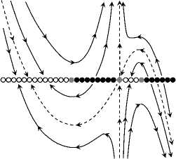
The classification of the system (49) is presented in Tables 5, 6 and in Fig. 4.

Table 5

Classification of the system (49) in a neighborhood of the node x = y = 0 in the space of small parameters v ₄ , v ₅ , and e ₄ . Here 5 21 = 5 2 ( v 5 , v ₄ , — e ₄ ).

The classes are written in the form g _w(_{ε 4} )_{, w}(_{δ 21} ) , where the function w is defined by (29)

Class (g 11 ) (g 12 ) = (a 1 )	C a 2 a 2 > 0, a 2 = 1 ( node )	onditio sgn ε 4 1 1 — 1 — 1	s sgn δ 21 1 — 1 1 — 1	E ε 4 α 3 α 3 — a 3 — a 3	xamp ( α >  0) ν 4 α 2 α 2 α 2 α 2	le ν 5 3 α α — 3 a — a
(g 21 )
(g 22 ) = (a 1 )
(g 01 )		0	1	0	— a 2	α
(g 02 ) = (a 0 )		0	— 1	0	α 2	α

Table 6

Classification of the system (49) in a neighborhood of the saddle x = y = 0 in the space of small parameters v ₄ , v ₅ , and £ 4 . Here 5 21 = 5 2 (v ₅ , v ₄ , — e ₄ ), n o = - (1 - 3a 2 ) £ 4 , П1 = 1 _l ^{- 3} a ² v₄, П2 = 1 ^- 3 ^{a 3} V5. The classes are written in the form ( hv²/”⁴,  ,_л  3,

η1      1-a2 4 , η2     1-2a2 5 .                                                           w(ε4), w(δ21 ) , where v2 and v4 are the components of the separatrix-intersection vector (28), and the function w is defined by (29)

Class (h 2111 ) (h 3201 )	a 2 a 2 <  0 (saddle)	Condi sgn ε 4 1 — 1	tions sgn δ 21 1	v 2 2 3 2	v 4 1 0 1	Examp η 0 — 6 a 3 6 α 3 4 a 4 2 (3 - a 2 ) 2    3	le ( α >  0) η 1 α 2 11 α 2 — 3a 2	η 2 4 α 6 α 0
(h 1201 )
						(1 - 3 a 2 ) 2 α
(h 1202 ) = (c 1 )			— 1	1	0	4 α 3	5 α 2	2 α
(h 2001 )		0	1	2	0	0	2 α 2	3 α
(h 1011 )				1	1		— 2 a 2 2 α 2 2 - 8 a 2 +7 a 2 2 α 2	α 2 α 1 - 2 a 2 α
(h 0001 )				0	0
(h 0002 ) = (c 0 )			— 1	0	0

Theorem 3. In the classification of the system (49) , all classes not listed in Tables 5 and 6 are empty:

(h 30 ),   (h 10 ), (h 10 ), (h 21 ),                                     (52)

(h 3Q ),    (h 3Q ),    (h ?2 ),    (h 22 ),    (h 2Q ),    (h Q2 ).                            (53)

The authors thank the two anonymous reviewers for their valuable comments.

Model systems (a) — (h) derived from equations (20) for which the codimension of degeneracy does not exceed two.

The symbols a j denote new coefficients, while ε j and ν j denote new small parameters. The matrix M is defined by (22)

Table 7

General conditions	Truncated system		Additional conditions		Model system			№
a 10 = 0	(30)	x = ( a io x + a oi y) (e o + y) y = (a io x + a oi y) (e o + y)	det M >  0 trM = 0	d M >  0 d M <  0	(32)	x = (a i x - y) • (e i + y) y = x • (e i + y)           _	a 2 i > 4 a 2 < 4 a i = 0	(a) (b)
a 10 = 0 a 10 = a 01 a 20 a 01 = 0	(35)	x = awx (e o + y) y = (^ i x + a oi y + a 2o x 2> • (e o + y)	det M <  0 a io a oi > 0		(32) (37)	x = (a i x + y) • (e i + y) y = x • (e i + y) x = a 2 x (e 2 + y) X/ = (v i x + y + x2) • • (e 2 + y)	a 2 > 0 a 2 = 1	(c) (d)
			a io a oi < 0				a 2 < 0	(e)
a io = 0 a io = a oi a 20 a 01 = 0	(42)	x = ( a io x + ^ 3 x + amy)- • (e o + y) y = (^ x + a oi y + ^ o y+ +a 2o x 2 ) • (e o + y)	—		(43)	x = (x + V 2 x + y) (e 3 + y) y/ = (v 3 x + y + x2) (e 3 + y)		(f)
a io = 0 a 20 = 0 a 30 a 0i = 0	(47)	x = a io x (e o + y) !/ = (^ i x + a oi y+ +^x2 + a 3o x 3 ) (e o + y)	a io a oi > 0		(49)	x = a 2 x (e 4 + y) y = (v 4 x + y + V 5 x 2 + +x 3 ) • (e 4 + y)	a 2 > 0 a 2 = 1	(g)
			a io a oi < 0				a 2 < 0	(h)

Classification of Dynamical Systems Near a Cosymmetric Equilibrium                    99

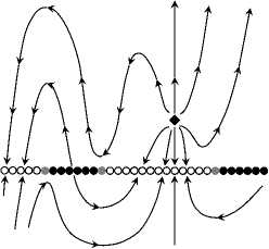
(g 11 )

⁽g 01 )

⁽g 21 )

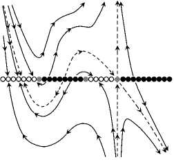
(h 11 )

(h 20 )

(h 30 )

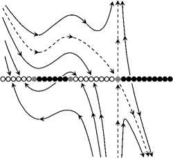
(h 20 )

(h 01)№

Fig. 4. Phase portraits of the model system (49) corresponding to the classification in Tables 5 and 6.