Coefficients identification in fractional diffusion models by the method of time integral characteristics

The fractional calculus [1-3] provides efficient tools for mathematical modelling of various processes. Differential equations with fractional derivatives of different kinds (so-called fractional differential equations) represent an important part of mathematical models used for investigation of processes with nonlocal spatial effects and memory [4-6]. Such processes are frequently observed in complex systems and inhomogeneous media. Anomalous diffusion processes form a wide class of such phenomena, and appropriate fractional diffusion equations have been much studied [7-10]. These equations permit the useful mathematical description of subdiffusion and superdiffusion processes in which the mean square displacement of a particle is described by a power law with an exponent not equal to one contrary to the classical Gaussian diffusion process.

However, the lack of initial data for a simulated process is one of the important problem of the theory of fractional differential equations which limit the practical use of such equations. In particular, a fractional diffusivity (or an anomalous diffusion coefficient) and orders of fractional differentiation are the required initial data for fractional anomalous diffusion equations. So, an important problem of fractional parameters identification arises. This problem leads to different mathematical formulations of inverse coefficient problems. It is necessary to note that the problem of identification of the order of fractional differentiation does not have an analog in the classical theory of inverse problems for integer order differential equations. Thus, new methods and algorithms of identification should be developed.

The integral characteristic methods [11-13] give simple and efficient algorithms of constant coefficients identification applicable to the linear partial differential ecpiations. These methods were efficiently used for identification of thermal properties of different materials [11,12]. On the basis of this methods, several non-destructive testing instruments for automatic identification of conductivity, heat capacity and thermal diffusivity was developed [14]. Subsequently, methods of integral characteristics were enhanced to inverse problems for different diffusion models. In particular, the diffusivity and drift coefficient have been successfully calculated for a model of the radiation-stimulated diffusion accompanying ion implantation processes [15,16].

The method of time integral characteristics [13] is one of the integral characteristic methods. In [17] the explicit integral representations for a constant anomalous diffusivity and the order of fractional differentiation have been derived using this method. These representations are based on the integral Laplace transform in time for a concentration function which is measured by time at the boundary and several inner points of calculation domain. In spite of all advantages of an explicit analytical form, these representations require that the concentration function must be known in the strictly determined inner points. This limitation restricts the practical use of these integral representations. Nevertheless, the restriction can be overcome by numerical algorithms. In this paper, the appropriate numerically-analytical algorithms based on the time integral characteristic method are proposed. These algorithms are implemented in the AD-TIC package for the Maple software. The functionality of this package is also briefly discussed.

1.    Formulations of Inverse Problems

Consider a set of fractional anomalous diffusion equations

D a u = ku xx + f ( t ) g ( x ) , x E ( a,b ) , t >  0 , a E (0 , 2) .

Here D a u is a left-sided fractional derivative of function u with respect to t of order a. The Riemann - Liouville D a u and Caputo C D a u time-fractional derivatives will be used as D a u . The difinitions of these fractional derivatives are as follows:

n

Dαu ≡     In-αu t      ∂tn t

D^au = I_t^t-a (   )

t t       ∂tn

1 dⁿ Г t    u ( x,t )

Г( n - a ) dt n J_o ( t V ' t + ^T,

1 Г t 1        dⁿu ( x,T )

Г( n - a ) J_o ( t - T ) a-n +¹    dT n    d^T'

Here Г( z ) is the Gannна function, n = [ a ] + 1 and

Dn^u =

¹       [ t    ^{u ( x,T} )    ,

Г(n - a) Jo (t - t)a-t+1 T is the left-sided time-fractional integral of order n — a.

Equation (1) with a E (0 , 1) can be used as a mathematical model for subdiffusion procesess, and with a E (1 , 2) as a model for diffusion-wave transfer. In the limiting case of a = 1 this equation coinsides with the classical diffusion equation, and for a = 2 it coincides with the classical wave equation.

Initial and boundary conditions are necessary for unique solvability of equation (1). The form of the initial conditions is defined by the type of fractional derivative. If the Riemann - Liouville fractional derivative (2) is used in equation (1) then the appropriate initial conditions have the form

In au|t=0 = фo(x), x G (a,b),   a G (0, 2),(4)

Da-1 u|t=o = фi(x), x G (a,b),   a G (1, 2).(5)

For the Caputo fractional derivative (3) the initial conditions have the form ult=0 = фo(x), x G (a,b), a G (0, 2),(6)

utlt=o = фi(x), x G (a,b), a G (1,2).(7)

In this paper, the boundary conditions of the first kind will be used:

u(a,t)= ua(t), u(b,t)= ub(t),   t> 0.(8)

In [9] it was proved that unique solutions exist for initial-boundary problems (1), (4), (5), (8) and (1), (6) - (8) if all functions in (4) - (7) and function t^n-af ( t ) are continuous functions in their domains of definition, and the following consistency conditions hold:

lim I n X ( t ) = ф o ( a ) ,   lim I n ^au_b ( t ) = ф o ( b );

t → 0                         t → 0

lim D a ¹ u a ( t ) = ф ₁( a ) ,   lim D 8 ^{- 1} u b ( t ) = ф ₁( b )

t→0 t                        t→0 t if the Riemann - Lioville fractional derivative is used in equation (1), and lim ua (t) = ф o( a), t→0

lim u a ⁽ t ) = Ф i ⁽ a ) , t → 0 ^a

lim u b ( t ) = ф o ( b );

t → 0

lim u b ⁽ t ) = ф i ⁽ b )

t → 0

if the Caputo fractional derivative is used. Further, we assume that these consistency conditions hold.

Now, let us formulate the inverse coefficient problem for identification of the diffusivity k and the order of fractional differentiation a. We assume that the appropriate initial conditions (4), (5) or (6), (7) and the boundary conditions (8) are known. Then the corresponding direct problems are solvable for all k >  0 and a G (0 , 2). An additional information about diffusion process is necessary for solving an inverse problem. Therefore, the concentration function u ( x,t ) will be assumed to be known at the certain inner points x = l i of calculation domain, i.e.

u ( l i ,t )= u i ( t ) , l i G ( a,b ) , i = 1 , 2 ,...,n, n> 1 ,

where u i ( t ) are known functions. If only one parameter ( k or a ) should be calculated whereas another parameter is known then one function u ₁( t ) is enough for solvability of the inverse problem (in this case n = 1).

2.    Identification Algorithms

The time integral characteristic method is based on an integral transform in time domain. The Laplace transform is commonly used as a such transform. Taking the Laplace transform of the linear initial-boundary problem, one can obtain a linear ordinary differential ecpiation which can be solved analytically. Then the desired parameters can be found from this solution using an additional information about the process.

Denote by v* ( p ) the Laplace trans form of a, function v ( t ):

v* ( P ) = / e pt v ( t ) dt. 0

Taking transform (10) of initial-boundary conditions for ecpiation (1), we get the following boundary value problem for the linear ordinary differential ecpiation of the second order:

P^au* ^{( x,}p ) = ku Xx ⁽ x,p ) + h ⁽ x,p^,a ) ,                           (11)

u* ⁽ a,P ) = u* ⁽ P ) ,   u* ^{( b,}P ) = u* ⁽ P ) .                             (12)

Here

( f* ⁽ p ) g ⁽ x ^{) +} Ф o⁽ x ) ,              ^а e (o , ¹⁾ ,

[ f * ( P ) g ( x )+ ^ 1( x )+ P^ о ( x ) , a e (1 , 2)

if the Riemann - Liouville fractional derivative is used, and

(f* ⁽ P ) g ⁽ x ⁾⁺ P^{a 1} Ф o⁽ x ) ,                  a E ⁽⁰ , ¹⁾ ,

[ f * ( P ) g ( x ) + P^a- ¹ Ф o( x ) + P^{a- 2} Ф 1( x ) , a E (1 , 2)

if the Caputo fractional derivative is used.

The solution of problem (11), (12) is well-known and can be represented in the form sinh A(b — a)u* (x,p) = sinh A(b — x) ^a(p) + (kA) 1 У h(£, p, a) sinh A(£ — a)d^ +

+ sinh A ( x — a )

^u* ⁽ P ) +

( kA ) ^{- 1 b} x

h ( (,P,a ) sinh A ( b — ( ) d(

where A =   p^a/k.

Substituting the Laplace transforms of the known concentration functions (9) into (13), we get a system of algebraic ecpiations. The residual quadratic functional for this system has the form n

Ф( k,a,p ) = £( S i + KF . )² ,                       (14)

i =1

where K = k ¹

S i ( A,p ) = sinh A ( b — l i ) u a ( p ) + sinh A ( l i — a ) u* ( p ) — sinh A ( b — a ) u* ( p ) ,

F i ^{( A,}P )

( A ) ¹ [sinh A ( b — l i ) j

h ( C,P, a ) sinh A ( C — a ) d^ +

+ sinh

A ( l i — a)

l i

h ( (,P,a ) sinh A ( b — ( ) d(

if the Riemann - Liouville fractional derivative is used, and

S i ( A,p ) = sinh A ( b — l i ) u* a ( p ) + sinh A ( l i — a ) u* ( p ) — sinh A ( b — a ) u* ( p )+

+ A sinh A ( b — l i )

l i

a

[P 1 Ф o⁽ < ⁾⁺ P 2 Ф 1⁽ < )] ^{sinh A (} < ^— a ) ^d< +

+ A sinh A ( l i

^— a ) j [ P 1 Ф o⁽ < ⁾⁺ P 2 Ф i⁽ < )] ^{sinh A ( b —}< ) d(,

F i ^{( A,}P )

( A ) ¹ [sinh A ( b — l i ) У

f* ⁽ P ) g ⁽ < ) ^{sinh A (} < ^— a ) ^d< +

+ sinh

A ( l i — a)

l i

f * ⁽ p ) g ⁽ ( ) sinh ^{A (} b^— £ ) d(

if the Caputo fractional derivative is used.

As it follows from the analysis of the above formulas, in the case of homogeneous equation (1) (i.e. if f ( t ) g ( x ) = 0) considered with the Caputo fractional derivative, the desired parameters k and a are coupled in Ф bу A because in this case F i = 0 , i = 1 , 2 ,..., n. If equation (1) is considered with the Riemann - Liouville fractional derivative then the order of fractional differentiation a is also coupled with k in Ф bу A but the diffusivity k is also presented in Ф independeutly from A.

Thus, if equation (1) is considered with the Riemann - Liouville fractional derivative or it is the nonhomogeneous equation with the Caputo fractional derivative then the desired parameters k and a can be found from the solution of the system of equations which is derived from the necessary conditions of an extremum for function (14):

д Ф       д Ф

= 0 ,      =0 .

∂k      ∂α

In the case of homogeneous equation (1) with the Caputo fractional derivative, A is the only parameter which can be determined from the equation дФ m =0. ∂λ

Minimization of (14) as a function of parameters k and a by a numerical routine leads to computational difficulties since the order of fractional differentiation a is presented in Ф only as the power function p^a. Nevertheless, the pair ( k, A ) can be considered insted of the pair ( k, a ). Substituting (14) into (15) we get the following system

Ё⁽ S i + ^KF i ) (^+ ^KdF +^{2 KF}-) =⁰ • i =1

n

^( Si + KFi i=1

) (SI + K|Fi) ∂λ ∂λ

= 0 .

The explicit representation for K can be found from this system as

K = -

nn

S i F i          F i ²

i =1            i =1

Then we get a unique equation for A:

n

E

Si - Fi

(E«)(£?) If - j =1            j =1

j

j

-

s (E Т(е '0

=1           =1

= 0 .

In the case of homogeneous equation (1) with the Caputo fractional derivative condition (16) leads to a more simple equation for the parameter A evaluation:

^E S i ⁸i =0 . i =1

As a result, we get the following algorithm for identification of parameters k and a. Solving (18) or (19), one can find the parameter A . Then from the representation (17) the diffusivity k can Ire calculated. Finally, the order of fractional differentiation a can Ire calculated from A by known k.

If all initial data are known without any errors then the proposed algorithm gives exact values of parameters k and a for any value of Laplace variable p. Nevertheless, in practice the initial data (such as a concentration function) are usually obtained from the experiments and therefore is known approximately. Then the values of k and a will depend on the value of p . So, a new important problem arises: it is necessary to determine the value of p such that the errors of identification of k and a will be minimal. Note that in the time integral characteristic method the parameter p can be considered as a regularization parameter of the identification algorithm. Therefore, the value of p should be consistent with the errors of initial data.

3.    Estimation of the Laplace Variable

In the method of time integral characteristics the values of the Laplace variable p always belong to a finite interval [ p min , p _max] which is determined by the chosen numerical algorithm for the Laplace transform calculation and by the time intervals in which the initial data are known. An efficient numerical algorithm for the Laplace transform calculation is based on a quadrature which is derived from an expansion of the Laplace integral by the system of the orthogonal Laguerre polynomials [18]:

v. (p) = /“ e-. v (t) dt = 1 J ~ e-. v hE . 1 £ V У v (4*

0               ^p 0 ^pp7 ^p k =1 ^T k \^Ln ^{( T} k V ^pp 7

Here the quadrature points Tk are the roots of the Laguerre polynomial of degree

Ln (Tk)

If a, function v is known on the interval [0 , t then the minimal value of p can Ire found from a condition that all quadrature points should belong to this interval: p _min = T n /t.

All known values of a function v ( t ) should be used for a proper calculation of the Laplace transform by (20). Therefore, the quadrature points should cover the finite interval [0 , t ] in which the variation of this function is significant (we assume that t < t because the Laplace transformation can not be calculated correctly otherwise). Then we have pmax = T n /t.

Another case is also possible if v ( t ) ^ v 0 = const with t ^ to. Then t ^ to and t can be chosen from the equality |v ( t ) — v 0 | = A _v , where A _v is an estimation for the absolute error of the function v ( t ). In tins case the following rule can be accepted: let l and m be given positive integers and no less than l and m quadrature points belong to the intervals [0 , t ] and [ t, to ). correspondingh'. Then we have p _min = T l /t and p _max = T_{n - m}Jt.

If there is no information about the errors of initial data then the parameters k and a can be evaluated from the function A(p) by the least sqirare method for p E [pmin, pmax]. In such approach these parameters are found by minimization of the function pmax

— 2 In A ( p )]² dp.

Ф(k, a)= /    [a In p — In k pmin

Then we get the following explicit representations:

a =2

pmax pmin

In

A ( p ) ln pdp — ( p ^{max ln} p ^max _ p ^{min ln} p min — 1) P m max In A ( p ) dp \       ^p max    ^p min            / Pm min

X

( p max ^- p min

p min p max

ln

2 p max

p max ^- p min    p min

k = exp

( p max

p min

p max

) -- pmin

( a In p — 2 In A ( p )) dp

X

If the error bounds for initial data are known then the optimal value p opt of the Laplace variable p can be evaluated by minimization of the error bound estimation for the parameter A which is derived from (18) or (19).

Let the absolute errors bounds A u A f A g, A _ф 0, A _ф 1, A ^ 0, A ^ 1 corresponding to the functions u ( t,x ), f ( t ), g ( x ), ф ₀( x ), ф 1 ( x ), ф ₀( x ), ф 1 ( x ) be known. The following estimates are valid for the absolute errors of the Laplace transform functions:

|u*(p,x) — u*(p,x) |< —,     f(p) — f*(p) < A, pp where u, f and U, f are correspondingly exact (unknown) and approximate (known) values of the functions u and f. Then the estimate of the absolute error for A derived from (18) has the form

n

^A A <  | ^Ja | 1 ^ ^{[ lJ} S i ^{1 A} S i + ^lJ F i ^{1 A} F i + S + ^KF i ^{| (A} dS i + K ^A dF i ^)] = ^A A ⁽ p ) ,    (23)

i =1

where nn ja = ^^ [52i + (Si + KFi)52i] — 52 ^^ Fi2, Jsi = 5Fi — 51i, JFi = (Si + 2KFi)5 — K51i, i=1                                 i=1

∂S ∂F        ∂ ² S     ∂ ² F         ^{n     - 1 n} ∂F

5 1 i = W + K m i ’ 5 2 i =    + K -y^ i , 5 = FTf, ²        KF ^A

∂λ ∂λ         ∂λ2     ∂λ2              i              ∂λ i=1          i=1

S i ∂S i

K ∂λ

)

and K is evaluated by (17). In addition, af = A a sinh AH—) sinh Alb—Ш sinh AH—1+

F i A ²               2               2               2

+4^a f pλ

li sinh A(b — li) / \g(£) | sinh A(£ — a)d£ + sinh A(li

a

l

• - a ) / \g ( £ ) I sinh A ( b - £ ) d£ l i

^A dF i

= -2 A h sinh λ ²

^b—a sinh ^A ( l i —a ) sinh ^b—^lA x

and

x

[( li — a ) coth

A ( li — a ) 2

+ ( b — l i ) coth

+ ""V2 I [ A ( b — l i ) cosh A ( b pλ ²

+ [ A ( l i — a ) cosh A ( l i —

+ A sinh A ( b —

—

^A-^ + ( b - a )coth A ( b

—

• a ) — d] +

l i

• l i ) — sinh A ( b - l i )]      \g ( £ ) \ sinh A ( £

a

— a ) d£ +

• a ) — sinh A ( li — a )] / \g ( £ ) \ sinh A ( b — £ ) d£ +

li li

• l i ) / \g ( £ ) \ ( £ ~ a ) cosh A ( £ - a ) d£ +

a

+ A sinh A ( l i

• ^—a ) y i \g ^{( £} ) \ ⁽ b -^{£ )cosh a (} b -^£ ) d^£^,

A_s. = 4 ^{A u} sinh ^{A (} b  a ) cosh

S i p           2

A ( b -l i ) ---2---cosh

^{A (} l i ^— a )

,

A dS i = — [( b — l i ) cosh A ( b i _p

—

l i ) + ( l i — a ) cosh A ( l i

— a ) + ( b — a ) cosh A ( b — a )] ,

_A = F \f* ( P ) I A g + A у 0 ,

[ \f* ^{( p} ) \ ^A g + ^{p A} У 0 + ^A У 1 , if the Riemann - Liouville fractional derivative is used,

a G (0,1); a G (1,2), and

^A S i = 4 ^sinh

A ( b — a )

p A u cosh

AA —» cosh A H -

A dSi = —u [( b — a ) cosh A ( b — a ) + ( b — i _p

+ ^{P A ф 0 + A ф} 1 [( b - a ) cosh A ( b - a ) — p ²

—

^a ) +

+ ( p A ф 0 + A ф 1 ) sinh

• l i )    cosh A ( b — l i ) + ( l i

( b — l i ) cosh A ( b — l i )

^{A ( b} — l i ) sinh ^{A (} l i — a )

,

—

—

• a ) cosh A ( l i — a )] +

( l i — a ) cosh A ( l i — a )] ,

A h = \f * ( P ) | A g if the Caputo fractional derivative is used.

The value of p = p opt such that

A a (Popt ) =    min   A a (p), p∈[pmin,pmax]

where the estimate A _A ( p ) is determined by (23) is called an optimal value of the Laplace variable p. Note th at since A _A ( p ) >  0. for a, finite interval [ p min , p max ] the positive value of p opt always exists.

Thus, the solution of inverse coefficient problem for ecpiation (1) is represented by the values of k and a which are calculated from A ( p_opt ) and representation (17).

4.    AD-TIC Package

The proposed algorithms from Sections 2 and 3 are implemented in the AD-TIC package for the math software Maple [19]. Employment of the Maple software permits to save the analytical evaluation for the most parameters of identification algorithms such us the estimate A _A ( p ) from (23), etc. This approach also permits the analytical representation of initial data in the graphical user interface and enables the access to all special functions in the Maple library.

The AD-TIC is a Maple package which includes a set of the Maple procedures. All these procedures are divided into four different groups:

• 1)    computational routines, which implement the proposed algorithms of parameters identification;

• 2)    input/output routines,

• 3)    postprocessing routines, which realize an additional processing of identification results,

• 4)    routines of graphical user interface.

The graphical user interface of the AD-TIC package was created using the Maplets technology of the Maple software. It contains several interactive forms. The Main Form is used for creating a calculation task in the work project format. The necessary functions of initial data (such as initial conditions, boundary conditions, the source function of the fractional diffusion equation) can be defined in explicit analytical forms in the Maple notation or by the tables with appropriate numerical values which are saved in the text files. If a function is defined by the table then a spline approximation is used. The order of spline approximation can be changed by user (the cubic spline approximation is used as a default setting). All fields of the Main Form are protected against incorrect data entry. Initial data are saved in the structural text file of the special format " .tic". An existing project file can be loaded from the Main Menu.

The AD-TIC package can be used for identification of the fractional diffusivity k and the order of fractional differentiation a for the fractional anomalous diffusion equation (1) with the Riemann - Liouville (2) and Caputo (3) fractional derivatives. The subdiffusion (a E (0 , 1)) and diffusion-wave ( a G (1 , 2)) equations are allowed. Two required parameters can be evaluated simultaneously as well as a single parameter identification ( k or a ) is available. The single coefficient k can be evaluated by the AD-TIC package for two limited cases of the classical diffusion equation (with a = 1) and the classical wave equation (with a = 2).

The known time concentration functions at several inner points of a calculation domain are used as initial data for identification. The values of coordinates of these inner points

ИЗ

(up to five) are entered in the appropriate fields of the Main Form of the package. The values of concentration functions are entered in the table format and are saved in the text files.

If the absolute error bounds for initial data are known then its values can also be entered in the appropriate fields of the Main Form. In this case the identification algorithm with p opt evaluation by minimization of (23) is available. Otherwise, the identification algorithm based on the least square method with averaging by the variable p E [ p _min , p _max] is used. All identification algorithms implemented in the AD-TIC package have several inner parameters and their values can be changed by user.

Now let us consider two test examples which were used for the verification of the AD-TIC package.

Example 1. The homogeneous subdiffusion equation (1) with the Riemann - Liouville fractional derivative was considered in the interval x E [0 , 1]. The initial condition (4) and boundary conditions (8) were chosen as

Ф o( x ) = (1 ~ x )³;       u o( t ) = 1 + t- ⁰ , ² e- ⁵ t ;       u i( t ) = 0 .

Using the finite difference method, a numerical solution of this initial-boundary value problem was obtained for the following numerical values of parameters: k = 1, a = 0 , 85. This solution at the three points 1 1 = 0 , 25, 12 = 0 , 5 and 1 3 = 0 , 75 was employed as initial data for the inverse coefficient problem. To simulate experimental errors, this solution was perturbed by the normally distributed random noise with zero mean. The variance of this noise was calculated from the condition that the absolute error of the concentration function does not exceed 5 %, i.e. A _u = 0 , 05.

The AD-TIC package was used for identification of k and a. The identification algorithm with p opt evaluation by minimization of (23) was chosen. Thirty quadrature points ( n = 30) were used for the numerical Laplace transform calculation by (20). The following numerical values of the boundaries for the Laplace variable p have been found: p min = 7 , 86 arid p _max = 34 , 97. Figure 1 shows the curve of dependence of A д оп p. It can Ire seen that this curve has a minimum at the inner point of the interval [ p _min , p _max]. This point corresponds to the optimal value of the Laplace variable p_opt = 22 , 82. Using this optimal value, the following values of the diffusivity and the order of fractional differentiation have been obtained: k = 0 , 933 arid a = 0 , 823.

So, the proposed algorithm permits to identify the parameters of the anomalous subdiffusion equation with the Riemann - Liouville fractional derivative with an acceptable accuracy.

Example 2. As a second example, the nonhomogeneous diffusion-wave equation with the Caputo fractional derivative was considered. The problem parameters were as follows:

g ( x ) = x,   ф o( x ) = x ³ + sin( nx ) ,  ф 1( x ) = 0 ,  x E [0 , 1];

f ( t ) = - 1 ,  u o( t )=0 ,               u i( t ) = 1 ,   t >  0 .

The equation parameters were chosen as k = 0 , 166 and a = 1 , 3.

As in the previous example, a numerical solution of this initial-boundary value problem was calculated using the finite difference method. This solution at the points 1 1 = 0 , 25,

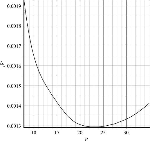
Fig. 1. The dependence of the absolute error estimate A a for the parameter A on the Laplace variable p

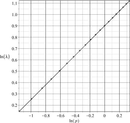
Fig. 2. The dependence of the parameter A on the Laplace variable p as a log-log plot

12 = 0 , 5 and 1 3 = 0 , 75 was used as initial data for the inverse coefficient problem without any perturbations. The absolute error bounds for the concentration function and other initial data were assumed to be unknown.

The AD-TIC package was used for identification of k and a. The identification algorithm based on the least square method with averaging by the variable p E [ p _min ,p _max] was used. A numerical calculation gave the following results for the boundaries of the

Laplace parameter interval: p _mj_n = 0 , 314 and p max = 1 , 398. The dependence of ln( A ) on ln( p ) for 25 vvalues of p is plotted on Figure 2. It can be seen that a straight line is a very good approximation for this data. The slope of this straight line corresponds to the following value of the order of fractional differentiation: a = 1 , 305. Using this value of a, the anomalous diffusivity k was evaluated as k = 0 , 165. Thus, the identification algorithm based on the least square method gives a good identification results for the case of small errors of the initial data.

Acknowledgements. This work was supported by the grant of the Ministry of Education and Science of the Russian Federation (contract No. 11.G3f.31.0042 with Ufa State Aviation Technical University and leading scientist Professor N.H. Ibragimov).