Computational experiment for one class of evolution mathematical models in quasi-Sobolev spaces

Let {Xk} C R+ Ite a monotone sequence such that lim Xk = + to. The quasi-Banach k→∞ space im = p={uk}: £ (x— кi)7<+to|

• ^ ^m         q ¹ /q

with a quasi-norm m ||u || = ( X k =1 ( Xk² |u_k|) )   , m E R is called a quasi-Sobolev space

• [1] . Obviously, for q E [1 , + to ) the spaces Im are Bana ch spaces; 1 0= l_qi and there is a dense and continuous embedding In in to Im for n > m and q E R₊.

Example 1. Let U = Im ^{+2 n} . F = I'm: Q_n ( X ). Rs ( X ) be polynomials of powers n and s ( n < s ) respectively with real coefficients, without common roots. Consider an operator L = Qn (Л) u = {Q_n ( Xk ) uk} . where {uk} E U. It is easy to see that the operator L E L ( U ; F ). Construct an operator M = Rs (Л) u = {Rs ( Xk ) uk} . It is easy to show that M E Cl ( U ; F ). dom M = Im ^{+2 s} . tlre L -spectrum a^L ( M ) of operator M consists of points Bk = Rs ( Xk )( Qn ( Xk )) ~ L k E N: Xk is not the root оf the polynomial Qn ( X ). Further we consider polynomials with the coefficients at the highest powers having opposite signs.

Definition 1. Vector-function u E C ¹(R₊; U), satisfying

Lu = Mu.                                (1)

pointwise is called a classical solution of this equation. The solution u = u(t) of (1) is called a solution to the weakened Cauchy problem (in sense of S.G. Krein), if in addition for uо E U lim u (t) = un. t-о 0+

holds.

If ker L = { 0 } then (1) is called a Sobolev type equation. Interest in Sobolev type equations has recently increased significantly [2-5], moreover, there arose a necessity for their consideration in quasi-Banach spaces. The need is dictated by the desire to fill up the theory as well as by the aspiration to comprehend non-classical models of mathematical physics in quasi-Banach spaces [6].

Since the Cauchy problem for the Sobolev type equation is not solvable for arbitrary initial data it is necessary to construct the phase space of equation as the set of admissible initial values containing all solutions of equation [2]. The phase spaces of evolution and dynamical Sobolev type equations were constructed earlier in Banach spaces [2]. These ideas were used to study one class of evolution Sobolev type equations in quasi-Banach spaces of sequences [6]. There was held an analytical investigation of the considered problem. A theorem of existence of unique solution was proved. Our gual is to develop an algorithm for the numerical solution of the problem and carry out computational experiments.

1.    Analytical Study of the Mathematical Model of One Class of Evolution Equations in Quasi-Banach Spaces

Lemma 1. [6] Operator M defined in example 1 is strongly L-sectorial.

Theorem 1. [6] Let operators M and L be defined as in example 1. Then

• (i)    operators L and M generate on spaces U and F degenerate holomorphic semigroups

{Ut : t E R₊ } and {Ft : t E R₊ } respectively given by

Ut

2 ni

I RL ( M ) e^dp

E L (U)

Ft

2 ni

LL ( M ) e^dp E L (F)

for t E R₊. where, thc contour Г C p^L ( M ) is sueh that \argp\ ^ 6 при p ^ to. p E Г.

• (ii)    there exist semigroup’s units which are the projectors P E L (U) a nd Q E L (F) given by

  P =| I ’- у

  kE N: k = I

  
  

if Xk is not the root of Q_n ( A ) for all k E N;

< ., ek > ek, If there exist I E N : X_l is the root of Q_n ( X ) ,

(the. projector Q has the. same. form), spHtUng the. quasi-Banach spaces U and F into direct sums

U=U⁰ Ф U¹ ,   F F Ф F¹ .

Definition 2. The set P C U is called a phase space of equation (1), if

• (1)    any solution u = u ( t ) of (1) lies In P polntwIse. he. u ( t ) E P for all t E R₊:

• (ii)    for all u о E P there exists a unique solution to (1), (2).

Theorem 2. [6] Let operators M and L be defined as in example 1. Then the subspace U¹ is a phase space о / (1), for arbitrary u ₀ E U¹ there exists a unique solution to (1), (2).

Definition 3. We say that solutions of (1) have exponential dichotomy, if

• (i)    the phase space of (1) can be represented as P = J¹Ф J², where J¹⁽²⁾ are invariant spaces of equation (1);

• (11)    for arbitrary u₀G J¹ (u₀G J²) soli.itlon u = u(t) of (1). (2) 1 s such that _U\\u(t)|| < C 1(uo)< ^-a(u \u(t) || > C₂(uo)e^at) for some a > 0 and all t G R₊ .

2.    Numerical Solution Algorithm

Theorem 3. [6] Let operators L,M G L(U; F) be defined as in example 1 and condition aL (M) П iR = 0 and there exists ^k G aL (M) with Re^k > 0

hold. Then solutions of (1) have exponential dichotomy.

Based on the theoretical results there was developed an algorithm for numerical solution of problem (1), (2), implemented in a software environment Maple 15.0. The program uses a phase space method [2].

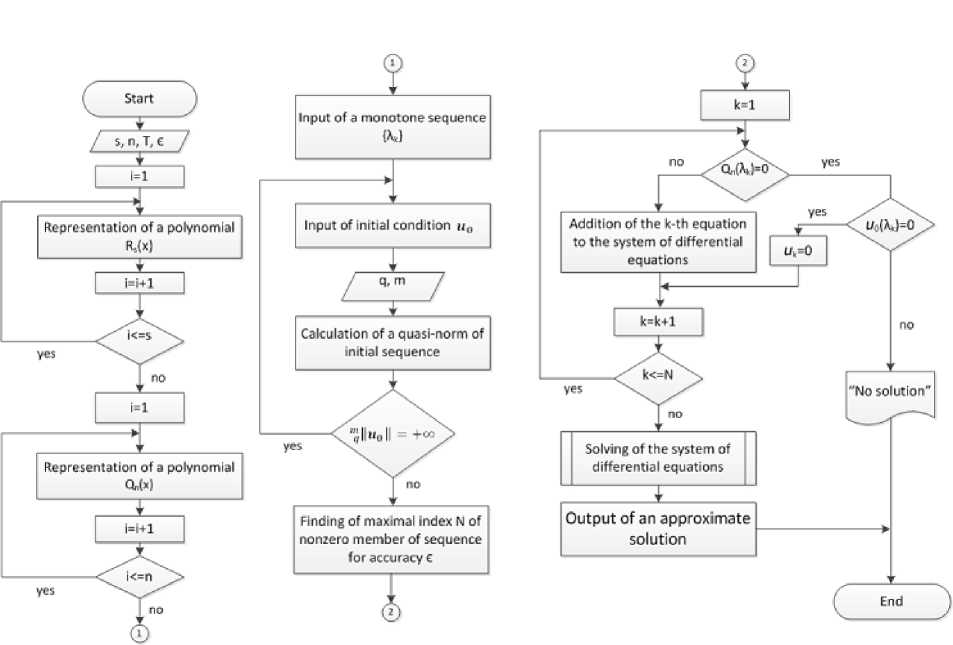
Fig. 1. A block diagram of algorithm

A numerical solution algorithm is shown in a block diagram in Fig. 1. The developed program allows you to:

• 1.    Enter the polynomials of the Laplace cpiasi-operator and consider one class of evolution equations in quasi-Sobolev spaces.

• 2.    Take into account degeneracy of equation and apply the phase space method.

• 3.    Find the necessary for the accuracy e number of nonzero members of approximate solution.

• 4.    Find and print the approximate solution of the problem.

• 5.    Get a graphical image of the components of received solution over time.

A detailed description of the algorithm (each block of the algorithm corresponds to one step):

Step 1. After the start of the program the user enters the powers of the polynomials s,n. the time period T : t E [0 , T ] and the accuracy of ari approximate solution e.

s

Step 2. In a cycle the polynomial Rs ( x ) =     dkxk is constructed.

k =1

n

Step 3. In a cycle the polynomial Qn ( x ) = ^) c_kxk is constructed.

k =1

Step 4- The monotone increasing sequence {Xk} is entered by user.

Step 5. The initial sequence u ₀ is set.

Step 6. Input of parameters of a quasi-norm of a quasi-Sobolev space.

Step 7. Calculation of a quasi-norm of the initial sequence.

Step 8. Checking if the quasi-norm of the initial sequence is infinite.

If the eighth step is true go to Step 5.

If the eighth step is false:

Step 9. Verification of number N of nontrivial components of approximate solution

T needed to take into account degeneracy and to obtain the accuracy e so th at J m^u (t) —

U _N ( t ) ^dt.

Step 10. In a cycle check if Qn ( Xk ) = 0, i.e. equation is degenerate.

If the tenth step is true:

Step 11. Check if initial data u ₀ belongs to the phase space of equation.

If the eleventh step is true:

Step 12. End of cycle by k.

If the eleventh step is false:

Step 13. Output the message:"There is no solution".

If the tenth step is false:

Step Ц. The к-th equation is a differential one. Add it to the system of differential equations to solve.

Step 15. End of cycle by k.

Step 16. Solve the system of differential equations to find the nontrivial components of an approximate solution.

Step П. The resulting approximate solution is put on the screen and displayed as graphs of the components of an approximate solution.

Step 18. End of program.

3.    Numerical Experiment

Let U = Im +^{2 n} , F = Im. Consider the Cauchy problem

u (0) = u 0 ,t E [0 ,T ] , u 0 E U,                               (4)

Qn (Л) u = Rs (Л) u.                               (5)

Example 2. It is required to find a numerical solution of problem (4) - (5) where

Q ₁( x ) = 2 — x, R ₂( x ) = x ² , Xk = k ² , u 0 _k = j. q = 0 , 5 , m = 1 , T = 0 , 5. e = 0 , 01 .

The program checks the condition m^u0| | = + to. Since it holds, there is no solution to the problem. The program gives output: "There is no solution".

Example 3. It is required to find a numerical solution of problem (4) - (5) where Q i( x ) =2 — x, R 2( x ) = x ² , Xk = k ² , u о k = ^. q = 0 , 5 , m = 1 , T = 0 , 5.

Depending on accuracy e we received the following results:

For e 1 = 0, 1, u1(t)=(et, 0,25 e-8t, 0,11 e-11 ’57t, 0,06 e-18’29t, 0,04 e-27’17t, 0, 0, ..., 0,...).

e 2 = 0, 01, u2(t)=(et. 0.25 e-8t. 0.11 e-11 ’57t. 0.06 e-18’29t. 0.04 e-27’17t. 0.03 e-38’12t. 0.02 e-51t 0.02 e-66t. 0.01 e-83t. 0.01 e-102t. 0.( 008 e-123t. 0.( 107 e-146t. 0.( 006 e-171 t. 0.( 105 e-198t. 0.004

e- ²²⁷ t

0, 0, ..., 0, ...J.

The graph of the solution is presented in Fig. 2.

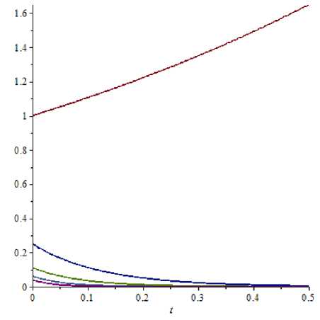
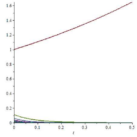
Fig. 2. Solution from example 3               Fig. 3. Solution from example 5

Example 4. It is required to find a numerical solution of problem (4) - (5) where Q 1( x ) = 4 — x, R 2( x ) = x ² , Xk = k ² , u о k = k 4 , . q = 0 , 5 , m = 1 , T = 0 , 5. e 1 = 0 , 1 . Equation (5) in this case is degenerate. Since the initial data do not belong to the phase space of equation the program gives output: "There is no solution".

Example 5. It is required to find the numerical solution of problem (4) - (5) where

Q 1( x ) =4 — x, R 2( x ) = x ² , Xk = kk².

u ⁰ k = -k² ’

if к = 2;

if k = 2.

Equation is degenerate ( Q ₁( X ₂) = 0) and initial data belong to the phase space of equation (5). For e = 0 , 01 we have

e( t )= et 0. 0.1 e- ¹¹ ’ ⁵⁷ t. 0.06 e- ¹⁸ ' ²⁹ t. 0.04 e- ²⁷ '17. 0.03 e- ³⁸ ' ¹² t. 0.02 e- ⁵¹6 0.02 e- ⁶⁶ t 0.01 e-83. 0.01 e- ¹⁰²6 0.( 108 e- ¹²³6 0.( 107 e- ¹⁴⁶6 0.( 106 e- ¹⁷¹6 0.( 105 e- ¹⁹⁸6 0.( 104 e- ²²⁷6 0.004 e- ²⁵⁸6 0.( 103 e- ²⁹¹6 0.( 103 e- ³²⁶4 0.( 103 e- ³⁶³6 0.( 103 e- ⁴⁰²6 0.( 102 e- ⁴⁴³6 0.( 102 e- ⁴⁸⁶ t. 0. 0,..., 0,... ).

The graph of the solution is presented in Fig. 3.

Example 6. It is recpiired to find a numerical solution of problem (4) - (5) where Q 2( x ) = 7 + x ² , R ₃( x ) = — 5 + x — 5 x ² — x ³ , Xk = k 4. u 0 _k = ^ 3. q = 0 . 5 , m = 1 , T = 0 . 5.

For e 1 = 0 , 1 ,

U 1( t )=( e^{- 1} , ^{25 1} , 0,13 e- ²⁰ ’ ^{39 1} , 0,04 e- ⁸⁵ ’ ^{9 1} , 0, 0,..., 0,...).

For e2 = 0, 01, ie2(t)=(e-1’25t, 0,13 e-20’39t, 0,04 e-85’91, 0,02 e-260t, 0 , 0,..., 0,...). The graph of the solution is presented in Fig. 4.

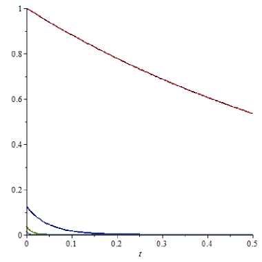
Fig. 4. Solution from example 6